Examples 2D
The following is a collection of example model setups, starting with an easy setup of the Barotropic vorticity equation and continuing with the shallow water model.
See also Examples 3D for examples with the primitive equation models.
2D turbulence on a non-rotating sphere
using SpeedyWeather
spectral_grid = SpectralGrid(trunc=63, nlev=1)
still_earth = Earth(spectral_grid, rotation=0)
initial_conditions = StartWithRandomVorticity()
model = BarotropicModel(; spectral_grid, initial_conditions, planet=still_earth)
simulation = initialize!(model)
run!(simulation, period=Day(20))
We want to use the barotropic model to simulate some free-decaying 2D turbulence on the sphere without rotation. We start by defining the SpectralGrid object. To have a resolution of about 200km, we choose a spectral resolution of T63 (see Available horizontal resolutions) and nlev=1 vertical levels. The SpectralGrid object will provide us with some more information
using SpeedyWeather
spectral_grid = SpectralGrid(trunc=63, nlev=1)
SpectralGrid:
├ Spectral: T63 LowerTriangularMatrix{Complex{Float32}}, radius = 6.371e6 m
├ Grid: 96-ring OctahedralGaussianGrid{Float32}, 10944 grid points
├ Resolution: 216km (average)
└ Vertical: 1-level SigmaCoordinatesNext step we create a planet that's like Earth but not rotating. As a convention, we always pass on the spectral grid object as the first argument to every other model component we create.
still_earth = Earth(spectral_grid, rotation=0)Earth{Float32} <: SpeedyWeather.AbstractPlanet
├ rotation::Float32 = 0.0
├ gravity::Float32 = 9.81
├ daily_cycle::Bool = true
├ length_of_day::Second = 86400 seconds
├ seasonal_cycle::Bool = true
├ length_of_year::Second = 31557600 seconds
├ equinox::DateTime = 2000-03-20T00:00:00
├ axial_tilt::Float32 = 23.4
└ solar_constant::Float32 = 341.25There are other options to create a planet but they are irrelevant for the barotropic vorticity equations. We also want to specify the initial conditions, randomly distributed vorticity is already defined
initial_conditions = StartWithRandomVorticity()StartWithRandomVorticity <: SpeedyWeather.AbstractInitialConditions
├ power::Float64 = -3.0
└ amplitude::Float64 = 1.0e-5By default, the power of vorticity is spectrally distributed with $k^{-3}$, $k$ being the horizontal wavenumber, and the amplitude is $10^{-5}\text{s}^{-1}$.
Now we want to construct a BarotropicModel with these
model = BarotropicModel(; spectral_grid, initial_conditions, planet=still_earth)The model contains all the parameters, but isn't initialized yet, which we can do with and then run it. The run! command will always return the prognostic variables, which, by default, are plotted for surface relative vorticity with a unicode plot. The resolution of the plot is not necessarily representative but it lets us have a quick look at the result
simulation = initialize!(model)
run!(simulation, period=Day(20))
Surface relative vorticity
┌────────────────────────────────────────────────────────────┐3.0f-6
90 │▄▄▄▄▄▄▄▄▄▄▄▄▄▄▄▄▄▄▄▄▄▄▄▄▄▄▄▄▄▄▄▄▄▄▄▄▄▄▄▄▄▄▄▄▄▄▄▄▄▄▄▄▄▄▄▄▄▄▄▄│ ┌──┐
│▄▄▄▄▄▄▄▄▄▄▄▄▄▄▄▄▄▄▄▄▄▄▄▄▄▄▄▄▄▄▄▄▄▄▄▄▄▄▄▄▄▄▄▄▄▄▄▄▄▄▄▄▄▄▄▄▄▄▄▄│ │▄▄│
│▄▄▄▄▄▄▄▄▄▄▄▄▄▄▄▄▄▄▄▄▄▄▄▄▄▄▄▄▄▄▄▄▄▄▄▄▄▄▄▄▄▄▄▄▄▄▄▄▄▄▄▄▄▄▄▄▄▄▄▄│ │▄▄│
│▄▄▄▄▄▄▄▄▄▄▄▄▄▄▄▄▄▄▄▄▄▄▄▄▄▄▄▄▄▄▄▄▄▄▄▄▄▄▄▄▄▄▄▄▄▄▄▄▄▄▄▄▄▄▄▄▄▄▄▄│ │▄▄│
│▄▄▄▄▄▄▄▄▄▄▄▄▄▄▄▄▄▄▄▄▄▄▄▄▄▄▄▄▄▄▄▄▄▄▄▄▄▄▄▄▄▄▄▄▄▄▄▄▄▄▄▄▄▄▄▄▄▄▄▄│ │▄▄│
│▄▄▄▄▄▄▄▄▄▄▄▄▄▄▄▄▄▄▄▄▄▄▄▄▄▄▄▄▄▄▄▄▄▄▄▄▄▄▄▄▄▄▄▄▄▄▄▄▄▄▄▄▄▄▄▄▄▄▄▄│ │▄▄│
│▄▄▄▄▄▄▄▄▄▄▄▄▄▄▄▄▄▄▄▄▄▄▄▄▄▄▄▄▄▄▄▄▄▄▄▄▄▄▄▄▄▄▄▄▄▄▄▄▄▄▄▄▄▄▄▄▄▄▄▄│ │▄▄│
˚N │▄▄▄▄▄▄▄▄▄▄▄▄▄▄▄▄▄▄▄▄▄▄▄▄▄▄▄▄▄▄▄▄▄▄▄▄▄▄▄▄▄▄▄▄▄▄▄▄▄▄▄▄▄▄▄▄▄▄▄▄│ │▄▄│
│▄▄▄▄▄▄▄▄▄▄▄▄▄▄▄▄▄▄▄▄▄▄▄▄▄▄▄▄▄▄▄▄▄▄▄▄▄▄▄▄▄▄▄▄▄▄▄▄▄▄▄▄▄▄▄▄▄▄▄▄│ │▄▄│
│▄▄▄▄▄▄▄▄▄▄▄▄▄▄▄▄▄▄▄▄▄▄▄▄▄▄▄▄▄▄▄▄▄▄▄▄▄▄▄▄▄▄▄▄▄▄▄▄▄▄▄▄▄▄▄▄▄▄▄▄│ │▄▄│
│▄▄▄▄▄▄▄▄▄▄▄▄▄▄▄▄▄▄▄▄▄▄▄▄▄▄▄▄▄▄▄▄▄▄▄▄▄▄▄▄▄▄▄▄▄▄▄▄▄▄▄▄▄▄▄▄▄▄▄▄│ │▄▄│
│▄▄▄▄▄▄▄▄▄▄▄▄▄▄▄▄▄▄▄▄▄▄▄▄▄▄▄▄▄▄▄▄▄▄▄▄▄▄▄▄▄▄▄▄▄▄▄▄▄▄▄▄▄▄▄▄▄▄▄▄│ │▄▄│
│▄▄▄▄▄▄▄▄▄▄▄▄▄▄▄▄▄▄▄▄▄▄▄▄▄▄▄▄▄▄▄▄▄▄▄▄▄▄▄▄▄▄▄▄▄▄▄▄▄▄▄▄▄▄▄▄▄▄▄▄│ │▄▄│
│▄▄▄▄▄▄▄▄▄▄▄▄▄▄▄▄▄▄▄▄▄▄▄▄▄▄▄▄▄▄▄▄▄▄▄▄▄▄▄▄▄▄▄▄▄▄▄▄▄▄▄▄▄▄▄▄▄▄▄▄│ │▄▄│
-90 │▄▄▄▄▄▄▄▄▄▄▄▄▄▄▄▄▄▄▄▄▄▄▄▄▄▄▄▄▄▄▄▄▄▄▄▄▄▄▄▄▄▄▄▄▄▄▄▄▄▄▄▄▄▄▄▄▄▄▄▄│ └──┘
└────────────────────────────────────────────────────────────┘-4.0f-6
0 ˚E 360 Woohoo! Something is moving! You could pick up where this simulation stopped by simply doing run!(simulation, period=Day(50)) again. We didn't store any output, which you can do by run!(simulation, output=true), which will switch on NetCDF output with default settings. More options on output in NetCDF output.
Shallow water with mountains
using SpeedyWeather
spectral_grid = SpectralGrid(trunc=63, nlev=1)
orography = NoOrography(spectral_grid)
initial_conditions = ZonalJet()
model = ShallowWaterModel(; spectral_grid, orography, initial_conditions)
simulation = initialize!(model)
run!(simulation, period=Day(6))
As a second example, let's investigate the Galewsky et al.[G04] test case for the shallow water equations with and without mountains. As the shallow water system has also only one level, we can reuse the SpectralGrid from Example 1.
using SpeedyWeather
spectral_grid = SpectralGrid(trunc=63, nlev=1)
SpectralGrid:
├ Spectral: T63 LowerTriangularMatrix{Complex{Float32}}, radius = 6.371e6 m
├ Grid: 96-ring OctahedralGaussianGrid{Float32}, 10944 grid points
├ Resolution: 216km (average)
└ Vertical: 1-level SigmaCoordinatesNow as a first simulation, we want to disable any orography, so we create a NoOrography
orography = NoOrography(spectral_grid)NoOrography{Float32, OctahedralGaussianGrid{Float32}} <: SpeedyWeather.AbstractOrography
└── arrays: orography, geopot_surfAlthough the orography is zero, you have to pass on spectral_grid so that it can still initialize zero-arrays of the correct size and element type. Awesome. This time the initial conditions should be set the the Galewsky et al.[G04] zonal jet, which is already defined as
initial_conditions = ZonalJet()ZonalJet <: SpeedyWeather.AbstractInitialConditions
├ latitude::Float64 = 45.0
├ width::Float64 = 19.28571428571429
├ umax::Float64 = 80.0
├ perturb_lat::Float64 = 45.0
├ perturb_lon::Float64 = 270.0
├ perturb_xwidth::Float64 = 19.098593171027442
├ perturb_ywidth::Float64 = 3.819718634205488
└ perturb_height::Float64 = 120.0The jet sits at 45˚N with a maximum velocity of 80m/s and a perturbation as described in their paper. Now we construct a model, but this time a ShallowWaterModel
model = ShallowWaterModel(; spectral_grid, orography, initial_conditions)
simulation = initialize!(model)
run!(simulation, period=Day(6))
Surface relative vorticity
┌────────────────────────────────────────────────────────────┐0.0001
90 │▄▄▄▄▄▄▄▄▄▄▄▄▄▄▄▄▄▄▄▄▄▄▄▄▄▄▄▄▄▄▄▄▄▄▄▄▄▄▄▄▄▄▄▄▄▄▄▄▄▄▄▄▄▄▄▄▄▄▄▄│ ┌──┐
│▄▄▄▄▄▄▄▄▄▄▄▄▄▄▄▄▄▄▄▄▄▄▄▄▄▄▄▄▄▄▄▄▄▄▄▄▄▄▄▄▄▄▄▄▄▄▄▄▄▄▄▄▄▄▄▄▄▄▄▄│ │▄▄│
│▄▄▄▄▄▄▄▄▄▄▄▄▄▄▄▄▄▄▄▄▄▄▄▄▄▄▄▄▄▄▄▄▄▄▄▄▄▄▄▄▄▄▄▄▄▄▄▄▄▄▄▄▄▄▄▄▄▄▄▄│ │▄▄│
│▄▄▄▄▄▄▄▄▄▄▄▄▄▄▄▄▄▄▄▄▄▄▄▄▄▄▄▄▄▄▄▄▄▄▄▄▄▄▄▄▄▄▄▄▄▄▄▄▄▄▄▄▄▄▄▄▄▄▄▄│ │▄▄│
│▄▄▄▄▄▄▄▄▄▄▄▄▄▄▄▄▄▄▄▄▄▄▄▄▄▄▄▄▄▄▄▄▄▄▄▄▄▄▄▄▄▄▄▄▄▄▄▄▄▄▄▄▄▄▄▄▄▄▄▄│ │▄▄│
│▄▄▄▄▄▄▄▄▄▄▄▄▄▄▄▄▄▄▄▄▄▄▄▄▄▄▄▄▄▄▄▄▄▄▄▄▄▄▄▄▄▄▄▄▄▄▄▄▄▄▄▄▄▄▄▄▄▄▄▄│ │▄▄│
│▄▄▄▄▄▄▄▄▄▄▄▄▄▄▄▄▄▄▄▄▄▄▄▄▄▄▄▄▄▄▄▄▄▄▄▄▄▄▄▄▄▄▄▄▄▄▄▄▄▄▄▄▄▄▄▄▄▄▄▄│ │▄▄│
˚N │▄▄▄▄▄▄▄▄▄▄▄▄▄▄▄▄▄▄▄▄▄▄▄▄▄▄▄▄▄▄▄▄▄▄▄▄▄▄▄▄▄▄▄▄▄▄▄▄▄▄▄▄▄▄▄▄▄▄▄▄│ │▄▄│
│▄▄▄▄▄▄▄▄▄▄▄▄▄▄▄▄▄▄▄▄▄▄▄▄▄▄▄▄▄▄▄▄▄▄▄▄▄▄▄▄▄▄▄▄▄▄▄▄▄▄▄▄▄▄▄▄▄▄▄▄│ │▄▄│
│▄▄▄▄▄▄▄▄▄▄▄▄▄▄▄▄▄▄▄▄▄▄▄▄▄▄▄▄▄▄▄▄▄▄▄▄▄▄▄▄▄▄▄▄▄▄▄▄▄▄▄▄▄▄▄▄▄▄▄▄│ │▄▄│
│▄▄▄▄▄▄▄▄▄▄▄▄▄▄▄▄▄▄▄▄▄▄▄▄▄▄▄▄▄▄▄▄▄▄▄▄▄▄▄▄▄▄▄▄▄▄▄▄▄▄▄▄▄▄▄▄▄▄▄▄│ │▄▄│
│▄▄▄▄▄▄▄▄▄▄▄▄▄▄▄▄▄▄▄▄▄▄▄▄▄▄▄▄▄▄▄▄▄▄▄▄▄▄▄▄▄▄▄▄▄▄▄▄▄▄▄▄▄▄▄▄▄▄▄▄│ │▄▄│
│▄▄▄▄▄▄▄▄▄▄▄▄▄▄▄▄▄▄▄▄▄▄▄▄▄▄▄▄▄▄▄▄▄▄▄▄▄▄▄▄▄▄▄▄▄▄▄▄▄▄▄▄▄▄▄▄▄▄▄▄│ │▄▄│
│▄▄▄▄▄▄▄▄▄▄▄▄▄▄▄▄▄▄▄▄▄▄▄▄▄▄▄▄▄▄▄▄▄▄▄▄▄▄▄▄▄▄▄▄▄▄▄▄▄▄▄▄▄▄▄▄▄▄▄▄│ │▄▄│
-90 │▄▄▄▄▄▄▄▄▄▄▄▄▄▄▄▄▄▄▄▄▄▄▄▄▄▄▄▄▄▄▄▄▄▄▄▄▄▄▄▄▄▄▄▄▄▄▄▄▄▄▄▄▄▄▄▄▄▄▄▄│ └──┘
└────────────────────────────────────────────────────────────┘-0.0001
0 ˚E 360 Oh yeah. That looks like the wobbly jet in their paper. Let's run it again for another 6 days but this time also store NetCDF output.
run!(simulation, period=Day(6), output=true) Surface relative vorticity
┌────────────────────────────────────────────────────────────┐9.0f-5
90 │▄▄▄▄▄▄▄▄▄▄▄▄▄▄▄▄▄▄▄▄▄▄▄▄▄▄▄▄▄▄▄▄▄▄▄▄▄▄▄▄▄▄▄▄▄▄▄▄▄▄▄▄▄▄▄▄▄▄▄▄│ ┌──┐
│▄▄▄▄▄▄▄▄▄▄▄▄▄▄▄▄▄▄▄▄▄▄▄▄▄▄▄▄▄▄▄▄▄▄▄▄▄▄▄▄▄▄▄▄▄▄▄▄▄▄▄▄▄▄▄▄▄▄▄▄│ │▄▄│
│▄▄▄▄▄▄▄▄▄▄▄▄▄▄▄▄▄▄▄▄▄▄▄▄▄▄▄▄▄▄▄▄▄▄▄▄▄▄▄▄▄▄▄▄▄▄▄▄▄▄▄▄▄▄▄▄▄▄▄▄│ │▄▄│
│▄▄▄▄▄▄▄▄▄▄▄▄▄▄▄▄▄▄▄▄▄▄▄▄▄▄▄▄▄▄▄▄▄▄▄▄▄▄▄▄▄▄▄▄▄▄▄▄▄▄▄▄▄▄▄▄▄▄▄▄│ │▄▄│
│▄▄▄▄▄▄▄▄▄▄▄▄▄▄▄▄▄▄▄▄▄▄▄▄▄▄▄▄▄▄▄▄▄▄▄▄▄▄▄▄▄▄▄▄▄▄▄▄▄▄▄▄▄▄▄▄▄▄▄▄│ │▄▄│
│▄▄▄▄▄▄▄▄▄▄▄▄▄▄▄▄▄▄▄▄▄▄▄▄▄▄▄▄▄▄▄▄▄▄▄▄▄▄▄▄▄▄▄▄▄▄▄▄▄▄▄▄▄▄▄▄▄▄▄▄│ │▄▄│
│▄▄▄▄▄▄▄▄▄▄▄▄▄▄▄▄▄▄▄▄▄▄▄▄▄▄▄▄▄▄▄▄▄▄▄▄▄▄▄▄▄▄▄▄▄▄▄▄▄▄▄▄▄▄▄▄▄▄▄▄│ │▄▄│
˚N │▄▄▄▄▄▄▄▄▄▄▄▄▄▄▄▄▄▄▄▄▄▄▄▄▄▄▄▄▄▄▄▄▄▄▄▄▄▄▄▄▄▄▄▄▄▄▄▄▄▄▄▄▄▄▄▄▄▄▄▄│ │▄▄│
│▄▄▄▄▄▄▄▄▄▄▄▄▄▄▄▄▄▄▄▄▄▄▄▄▄▄▄▄▄▄▄▄▄▄▄▄▄▄▄▄▄▄▄▄▄▄▄▄▄▄▄▄▄▄▄▄▄▄▄▄│ │▄▄│
│▄▄▄▄▄▄▄▄▄▄▄▄▄▄▄▄▄▄▄▄▄▄▄▄▄▄▄▄▄▄▄▄▄▄▄▄▄▄▄▄▄▄▄▄▄▄▄▄▄▄▄▄▄▄▄▄▄▄▄▄│ │▄▄│
│▄▄▄▄▄▄▄▄▄▄▄▄▄▄▄▄▄▄▄▄▄▄▄▄▄▄▄▄▄▄▄▄▄▄▄▄▄▄▄▄▄▄▄▄▄▄▄▄▄▄▄▄▄▄▄▄▄▄▄▄│ │▄▄│
│▄▄▄▄▄▄▄▄▄▄▄▄▄▄▄▄▄▄▄▄▄▄▄▄▄▄▄▄▄▄▄▄▄▄▄▄▄▄▄▄▄▄▄▄▄▄▄▄▄▄▄▄▄▄▄▄▄▄▄▄│ │▄▄│
│▄▄▄▄▄▄▄▄▄▄▄▄▄▄▄▄▄▄▄▄▄▄▄▄▄▄▄▄▄▄▄▄▄▄▄▄▄▄▄▄▄▄▄▄▄▄▄▄▄▄▄▄▄▄▄▄▄▄▄▄│ │▄▄│
│▄▄▄▄▄▄▄▄▄▄▄▄▄▄▄▄▄▄▄▄▄▄▄▄▄▄▄▄▄▄▄▄▄▄▄▄▄▄▄▄▄▄▄▄▄▄▄▄▄▄▄▄▄▄▄▄▄▄▄▄│ │▄▄│
-90 │▄▄▄▄▄▄▄▄▄▄▄▄▄▄▄▄▄▄▄▄▄▄▄▄▄▄▄▄▄▄▄▄▄▄▄▄▄▄▄▄▄▄▄▄▄▄▄▄▄▄▄▄▄▄▄▄▄▄▄▄│ └──┘
└────────────────────────────────────────────────────────────┘-8.0f-5
0 ˚E 360 The progress bar tells us that the simulation run got the identification "0001" (which just counts up, so yours might be higher), meaning that data is stored in the folder /run_0001. In general we can check this also via
id = model.output.id"0001"So let's plot that data properly (and not just using UnicodePlots.jl). $id in the following just means that the string is interpolated to run_0001 if this is the first unnamed run in your folder.
using NCDatasets
ds = NCDataset("run_$id/output.nc")
ds["vor"]
vor (192 × 96 × 1 × 25)
Datatype: Union{Missing, Float32} (Float32)
Dimensions: lon × lat × lev × time
Attributes:
units = 1/s
long_name = relative vorticity
_FillValue = NaN
Vorticity vor is stored as a lon x lat x vert x time array, we may want to look at the first time step, which is the end of the previous simulation (time = 6days) which we didn't store output for.
t = 1
vor = Matrix{Float32}(ds["vor"][:, :, 1, t]) # convert from Matrix{Union{Missing, Float32}} to Matrix{Float32}
lat = ds["lat"][:]
lon = ds["lon"][:]

using CairoMakie
heatmap(lon, lat, vor)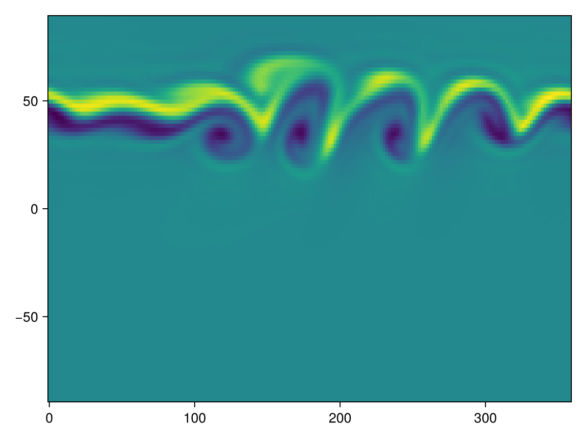
You see that in comparison the unicode plot heavily coarse-grains the simulation, well it's unicode after all! Here, we have unpacked the netCDF file using NCDatasets.jl and then plotted via heatmap(lon, lat, vor). While you can do that to give you more control on the plotting, SpeedyWeather.jl also defines an extension for Makie.jl, see Extensions. Because if our matrix vor here was an AbstractGrid (see RingGrids) then all its geographic information (which grid point is where) would directly be encoded in the type. From the netCDF file you need to use the longitude and latitude dimensions.
So we can also just do
vor_grid = FullGaussianGrid(vor)

using CairoMakie    # this will load the extension so that Makie can plot grids directly
heatmap(vor_grid, title="Relative vorticity [1/s]")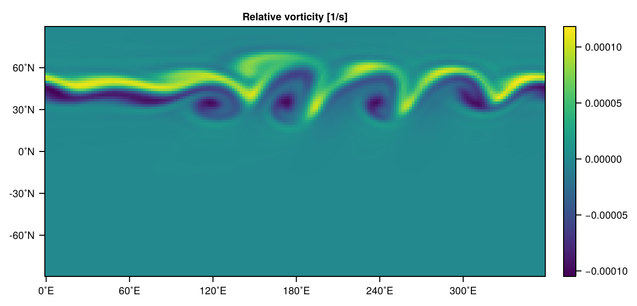
Note that here you need to know which grid the data comes on (an error is thrown if FullGaussianGrid(vor) is not size compatible). By default the output will be on the FullGaussianGrid, but if you play around with other grids, you'd need to change this here, see NetCDF output on other grids.
We did want to showcase the usage of NetCDF output here, but from now on we will use heatmap to plot data on our grids directly, without storing output first. So for our current simulation, that means at time = 12 days, vorticity on the grid is stored in the diagnostic variables and can be visualised with
vor = simulation.diagnostic_variables.layers[1].grid_variables.vor_grid
heatmap(vor, title="Relative vorticity [1/s]")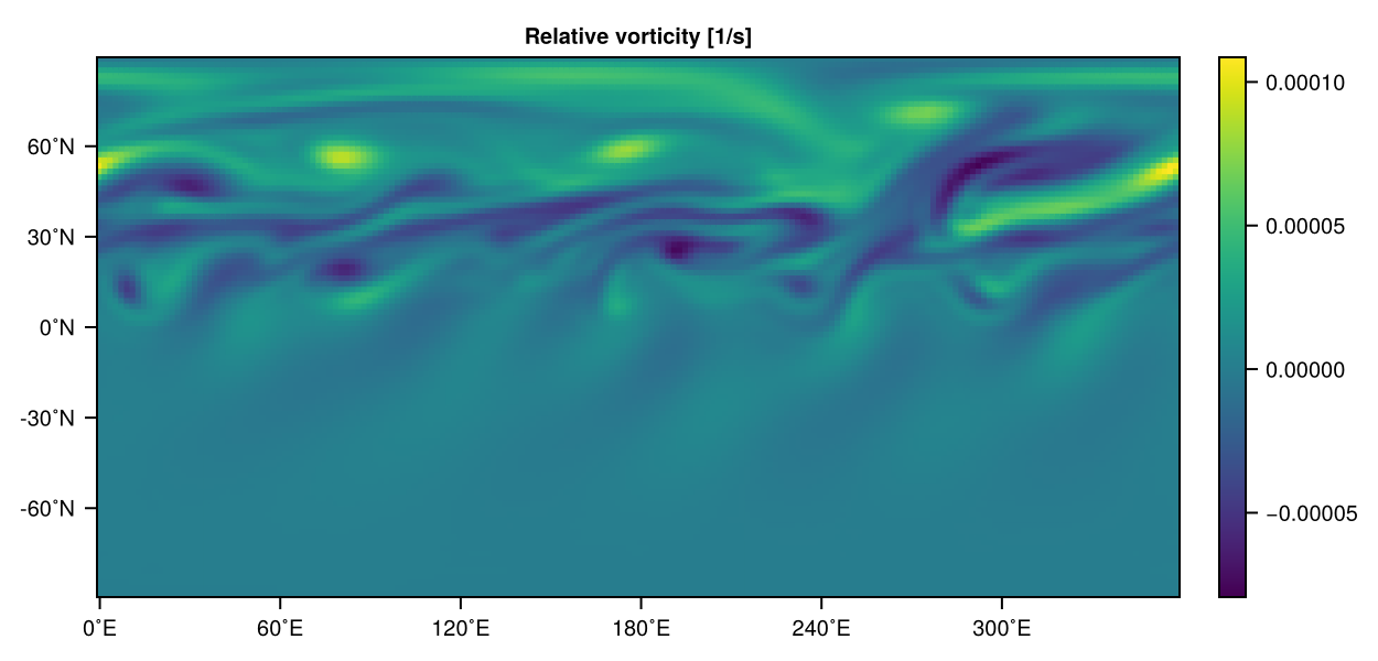
The jet broke up into many small eddies, but the turbulence is still confined to the northern hemisphere, cool! How this may change when we add mountains (we had NoOrography above!), say Earth's orography, you may ask? Let's try it out! We create an EarthOrography struct like so
orography = EarthOrography(spectral_grid)EarthOrography{Float32, OctahedralGaussianGrid{Float32}} <: SpeedyWeather.AbstractOrography
├ path::String = SpeedyWeather.jl/input_data
├ file::String = orography.nc
├ file_Grid::UnionAll = FullGaussianGrid
├ scale::Float64 = 1.0
├ smoothing::Bool = true
├ smoothing_power::Float64 = 1.0
├ smoothing_strength::Float64 = 0.1
├ smoothing_fraction::Float64 = 0.05
└── arrays: orography, geopot_surfIt will read the orography from file as shown (only at initialize!(model)), and there are some smoothing options too, but let's not change them. Same as before, create a model, initialize into a simulation, run. This time directly for 12 days so that we can compare with the last plot
model = ShallowWaterModel(; spectral_grid, orography, initial_conditions)
simulation = initialize!(model)
run!(simulation, period=Day(12), output=true)
Surface relative vorticity
┌────────────────────────────────────────────────────────────┐9.0f-5
90 │▄▄▄▄▄▄▄▄▄▄▄▄▄▄▄▄▄▄▄▄▄▄▄▄▄▄▄▄▄▄▄▄▄▄▄▄▄▄▄▄▄▄▄▄▄▄▄▄▄▄▄▄▄▄▄▄▄▄▄▄│ ┌──┐
│▄▄▄▄▄▄▄▄▄▄▄▄▄▄▄▄▄▄▄▄▄▄▄▄▄▄▄▄▄▄▄▄▄▄▄▄▄▄▄▄▄▄▄▄▄▄▄▄▄▄▄▄▄▄▄▄▄▄▄▄│ │▄▄│
│▄▄▄▄▄▄▄▄▄▄▄▄▄▄▄▄▄▄▄▄▄▄▄▄▄▄▄▄▄▄▄▄▄▄▄▄▄▄▄▄▄▄▄▄▄▄▄▄▄▄▄▄▄▄▄▄▄▄▄▄│ │▄▄│
│▄▄▄▄▄▄▄▄▄▄▄▄▄▄▄▄▄▄▄▄▄▄▄▄▄▄▄▄▄▄▄▄▄▄▄▄▄▄▄▄▄▄▄▄▄▄▄▄▄▄▄▄▄▄▄▄▄▄▄▄│ │▄▄│
│▄▄▄▄▄▄▄▄▄▄▄▄▄▄▄▄▄▄▄▄▄▄▄▄▄▄▄▄▄▄▄▄▄▄▄▄▄▄▄▄▄▄▄▄▄▄▄▄▄▄▄▄▄▄▄▄▄▄▄▄│ │▄▄│
│▄▄▄▄▄▄▄▄▄▄▄▄▄▄▄▄▄▄▄▄▄▄▄▄▄▄▄▄▄▄▄▄▄▄▄▄▄▄▄▄▄▄▄▄▄▄▄▄▄▄▄▄▄▄▄▄▄▄▄▄│ │▄▄│
│▄▄▄▄▄▄▄▄▄▄▄▄▄▄▄▄▄▄▄▄▄▄▄▄▄▄▄▄▄▄▄▄▄▄▄▄▄▄▄▄▄▄▄▄▄▄▄▄▄▄▄▄▄▄▄▄▄▄▄▄│ │▄▄│
˚N │▄▄▄▄▄▄▄▄▄▄▄▄▄▄▄▄▄▄▄▄▄▄▄▄▄▄▄▄▄▄▄▄▄▄▄▄▄▄▄▄▄▄▄▄▄▄▄▄▄▄▄▄▄▄▄▄▄▄▄▄│ │▄▄│
│▄▄▄▄▄▄▄▄▄▄▄▄▄▄▄▄▄▄▄▄▄▄▄▄▄▄▄▄▄▄▄▄▄▄▄▄▄▄▄▄▄▄▄▄▄▄▄▄▄▄▄▄▄▄▄▄▄▄▄▄│ │▄▄│
│▄▄▄▄▄▄▄▄▄▄▄▄▄▄▄▄▄▄▄▄▄▄▄▄▄▄▄▄▄▄▄▄▄▄▄▄▄▄▄▄▄▄▄▄▄▄▄▄▄▄▄▄▄▄▄▄▄▄▄▄│ │▄▄│
│▄▄▄▄▄▄▄▄▄▄▄▄▄▄▄▄▄▄▄▄▄▄▄▄▄▄▄▄▄▄▄▄▄▄▄▄▄▄▄▄▄▄▄▄▄▄▄▄▄▄▄▄▄▄▄▄▄▄▄▄│ │▄▄│
│▄▄▄▄▄▄▄▄▄▄▄▄▄▄▄▄▄▄▄▄▄▄▄▄▄▄▄▄▄▄▄▄▄▄▄▄▄▄▄▄▄▄▄▄▄▄▄▄▄▄▄▄▄▄▄▄▄▄▄▄│ │▄▄│
│▄▄▄▄▄▄▄▄▄▄▄▄▄▄▄▄▄▄▄▄▄▄▄▄▄▄▄▄▄▄▄▄▄▄▄▄▄▄▄▄▄▄▄▄▄▄▄▄▄▄▄▄▄▄▄▄▄▄▄▄│ │▄▄│
│▄▄▄▄▄▄▄▄▄▄▄▄▄▄▄▄▄▄▄▄▄▄▄▄▄▄▄▄▄▄▄▄▄▄▄▄▄▄▄▄▄▄▄▄▄▄▄▄▄▄▄▄▄▄▄▄▄▄▄▄│ │▄▄│
-90 │▄▄▄▄▄▄▄▄▄▄▄▄▄▄▄▄▄▄▄▄▄▄▄▄▄▄▄▄▄▄▄▄▄▄▄▄▄▄▄▄▄▄▄▄▄▄▄▄▄▄▄▄▄▄▄▄▄▄▄▄│ └──┘
└────────────────────────────────────────────────────────────┘-7.0f-5
0 ˚E 360 This time the run got a new run id, which you see in the progress bar, but can again always check after the run! call (the automatic run id is only determined just before the main time loop starts) with model.output.id, but otherwise we do as before.
id = model.output.id"0002"ds = NCDataset("run_$id/output.nc")Dataset: run_0002/output.nc
Group: /
Dimensions
time = 49
lon = 192
lat = 96
lev = 1
Variables
time (49)
Datatype: DateTime (Float64)
Dimensions: time
Attributes:
units = hours since 2000-01-01 00:00:0.0
calendar = proleptic_gregorian
long_name = time
standard_name = time
lon (192)
Datatype: Float64 (Float64)
Dimensions: lon
Attributes:
units = degrees_east
long_name = longitude
lat (96)
Datatype: Float64 (Float64)
Dimensions: lat
Attributes:
units = degrees_north
long_name = latitude
lev (1)
Datatype: Float32 (Float32)
Dimensions: lev
Attributes:
units = 1
long_name = sigma levels
u (192 × 96 × 1 × 49)
Datatype: Union{Missing, Float32} (Float32)
Dimensions: lon × lat × lev × time
Attributes:
units = m/s
long_name = zonal wind
_FillValue = NaN
v (192 × 96 × 1 × 49)
Datatype: Union{Missing, Float32} (Float32)
Dimensions: lon × lat × lev × time
Attributes:
units = m/s
long_name = meridional wind
_FillValue = NaN
vor (192 × 96 × 1 × 49)
Datatype: Union{Missing, Float32} (Float32)
Dimensions: lon × lat × lev × time
Attributes:
units = 1/s
long_name = relative vorticity
_FillValue = NaN
You could plot the NetCDF output now as before, but we'll be plotting directly from the current state of the simulation
vor = simulation.diagnostic_variables.layers[1].grid_variables.vor_grid
heatmap(vor, title="Relative vorticity [1/s]")
Interesting! The initial conditions have zero velocity in the southern hemisphere, but still, one can see some imprint of the orography on vorticity. You can spot the coastline of Antarctica; the Andes and Greenland are somewhat visible too. Mountains also completely changed the flow after 12 days, probably not surprising!
Polar jet streams in shallow water
Setup script to copy and paste:
using SpeedyWeather
spectral_grid = SpectralGrid(trunc=63, nlev=1)

forcing = JetStreamForcing(spectral_grid, latitude=60)
drag = QuadraticDrag(spectral_grid)

model = ShallowWaterModel(; spectral_grid, drag, forcing)
simulation = initialize!(model)
run!(simulation, period=Day(40))
We want to simulate polar jet streams in the shallow water model. We add a JetStreamForcing that adds momentum at 60˚N to inject kinetic energy into the model. This energy needs to be removed (the diffusion is likely not sufficient) through a drag, we have implemented a QuadraticDrag and use the default drag coefficient. Then visualize zonal wind after 40 days with
using CairoMakie

u = simulation.diagnostic_variables.layers[1].grid_variables.u_grid
heatmap(u, title="Zonal wind [m/s]")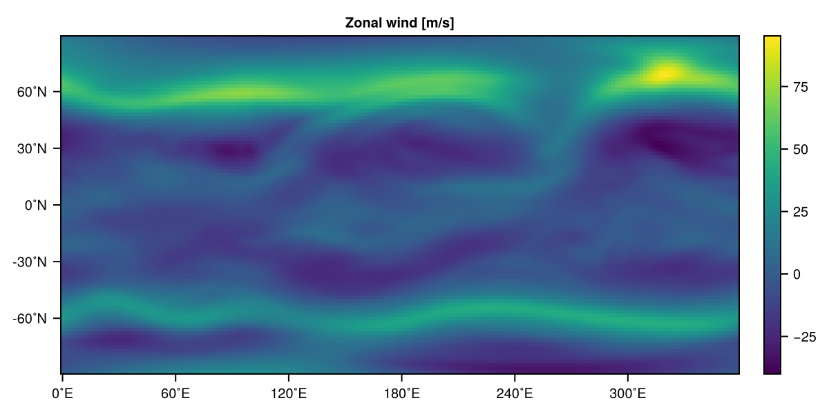
Gravity waves on the sphere
Setup script to copy and paste:
using SpeedyWeather
spectral_grid = SpectralGrid(trunc=127, nlev=1)

# model components
time_stepping = SpeedyWeather.Leapfrog(spectral_grid, Δt_at_T31=Minute(30))
implicit = SpeedyWeather.ImplicitShallowWater(spectral_grid, α=0.5)
orography = EarthOrography(spectral_grid, smoothing=false)
initial_conditions = SpeedyWeather.RandomWaves()

# construct, initialize, run
model = ShallowWaterModel(; spectral_grid, orography, initial_conditions, implicit, time_stepping)
simulation = initialize!(model)
run!(simulation, period=Day(2))
How are gravity waves propagating around the globe? We want to use the shallow water model to start with some random perturbations of the interface displacement (the "sea surface height") but zero velocity and let them propagate around the globe. We set the $\alpha$ parameter of the semi-implicit time integration to $0.5$ to have a centred implicit scheme which dampens the gravity waves less than a backward implicit scheme would do. But we also want to keep orography, and particularly no smoothing on it, to have the orography as rough as possible. The initial conditions are set to RandomWaves which set the spherical harmonic coefficients of $\eta$ to between given wavenumbers to some random values
SpeedyWeather.RandomWaves()RandomWaves <: SpeedyWeather.AbstractInitialConditions
├ A::Float64 = 2000.0
├ lmin::Int64 = 10
└ lmax::Int64 = 20so that the amplitude A is as desired, here 2000m. Our layer thickness in meters is by default
model.atmosphere.layer_thickness8500.0f0so those waves are with an amplitude of 2000m quite strong. But the semi-implicit time integration can handle that even with fairly large time steps of
model.time_stepping.Δt_sec450.0f0seconds. Note that the gravity wave speed here is $\sqrt{gH}$ so almost 300m/s, given the speed of gravity waves we don't have to integrate for long. Visualise the dynamic layer thickness $h = \eta + H + H_b$ (interface displacement $\eta$, layer thickness at rest $H$ and orography $H_b$) with
using CairoMakie

H = model.atmosphere.layer_thickness
Hb = model.orography.orography
η = simulation.diagnostic_variables.surface.pres_grid
h = @. η + H - Hb   # @. to broadcast grid + scalar - grid

heatmap(h, title="Dynamic layer thickness h", colormap=:oslo)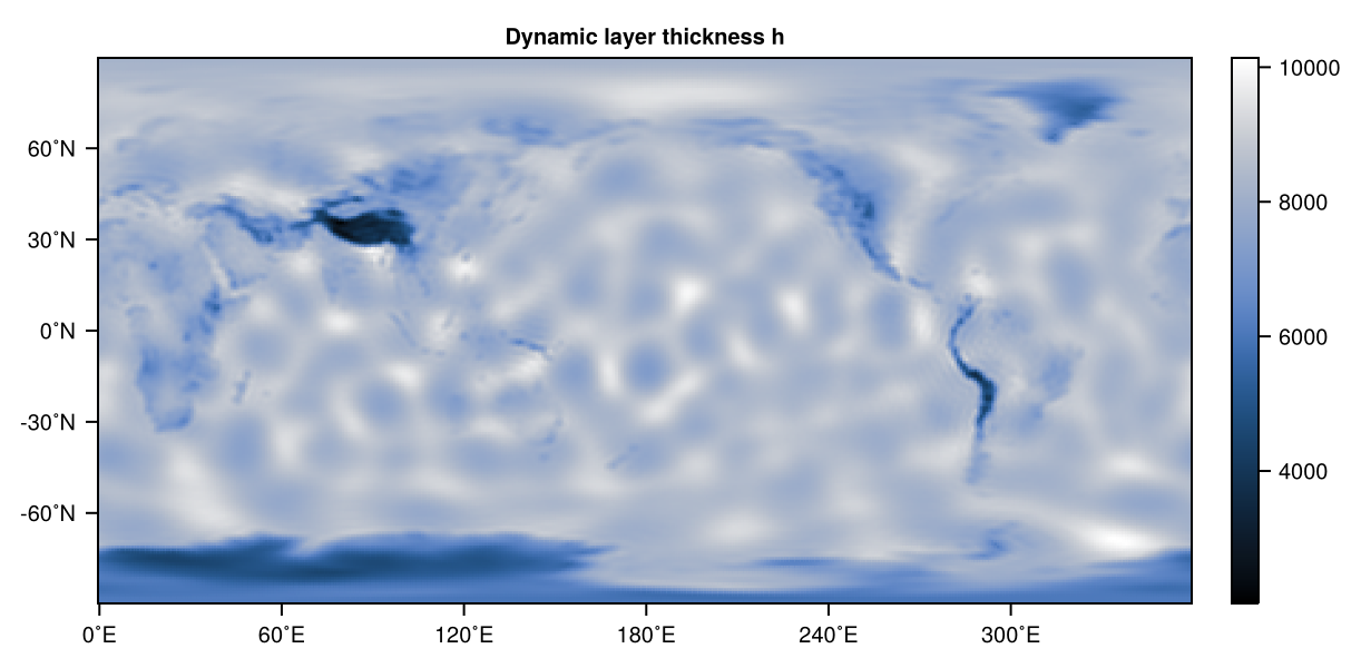
Can you spot the Himalayas or the Andes?
References
- G04Galewsky, Scott, Polvani, 2004. An initial-value problem for testing numerical models of the global shallow-water equations, Tellus A. DOI: 10.3402/tellusa.v56i5.14436