Initial conditions

The following showcases some examples of how to set the initial conditions for the prognostic variables in SpeedyWeather.jl. In essence there are three ways to do this

1. Change the arrays in simulation.variables.prognostic

2. Use the set! function

3. Set the initial_conditions component of a model

where 1 is a rather low-level and largely requires you to directly set the complex coefficients of the spherical harmonics (advanced!). So the set! function builds a convenient interface around 1 such that you don't have to know about details of grid or spectral space (see also Setting variables for more on set!). 3 then collects method 1 or 2 (or a combination of both) into a single struct to "save" some initial conditions for one or several variables, similar to the initial_conditions model component described in Creating model components. This lets you use predefined (inside SpeedyWeather or externally) initial conditions as easy as initial_conditions = RossbyHaurwitzWave(). Let us illustrate this with some examples where we will refer back those methods simply as 1, 2, 3.

Rossby-Haurwitz wave in a BarotropicModel

We define a BarotropicModel of some resolution without forcing and drag

using SpeedyWeather
spectral_grid = SpectralGrid(truncation=64, nlayers=1)
model = BarotropicModel(spectral_grid, forcing=nothing, drag=nothing)
simulation = initialize!(model)

Simulation{...} (2.93 MB)
├ variables::Variables{...} (498.44 KB)
└ model::BarotropicModel{...} (2.51 MB)

Now simulation.variables.prognostic contains already some initial conditions as defined by model.initial_conditions (that's method 3). Regardless of what those are, we can still mutate them before starting a simulation, but if you (re-)initialize the model, the initial conditions will be set back to what is defined in model.initial_conditions. We will illustrate the set! function now that conveniently lets you (re)set the current state of the prognostic variables:

The Rossby-Haurwitz wave () is defined as an initial condition for vorticity (which is the sole prognostic variable in the barotropic vorticity model) as

with longitude and latitude . The parameters are zonal wavenumber (order)  , frequencies   ,   . Now setting these initial conditions is as simple as

m = 4
ω = 7.848e-6
K = 7.848e-6

ζ(λ, θ, σ) = 2ω*sind(θ) - K*sind(θ)*cosd(θ)^m*(m^2 + 3m + 2)*cosd(m*λ)
set!(simulation, vorticity=ζ, step=1)

with only two difference from the mathematical notation. (1) SpeedyWeather's coordinates are in degrees, so we replaced with sind and cosd; and (2) To generalise to vertical coordinates, the function ζ(λ, θ, σ) takes exactly three arguments, with σ denoting the vertical Sigma coordinates. This is important so that we can use the same definition of initial conditions for the 2D barotropic vorticity model also for the 3D primitive equations. Furthermore we explicitly set here step 1, as, depending on the time stepper, prognostic variables may have more than 1 step, see Step dimension for more details. Leapfrog for example has 2 steps but it's important to set the initial conditions for step 1 here, not step 2.

One may filter out low values of spectral vorticity with some cut-off amplitude  , just to illustrate how you would do this (example for method 1)

c = 1e-10       # cut-off amplitude

# get_step to view the correct step index
vor = get_step(simulation.variables.prognostic.vorticity, 1)
low_values = abs.(vor) .< c
vor[low_values] .= 0

which is just treating vor as an array of something and tweaking the values within!

Let us illustrate these initial conditions. set! will set the initial conditions in spectral space, taking care of the transform from the equation defined in grid coordinates. So to show vorticity again in grid space we transform back

# use [:, 1] to read out all horizontal point but only the first and only vertical layer
vor_grid = transform(vor[:, 1])

using CairoMakie
heatmap(vor_grid, title="Relative vorticity [1/s] of Rossby-Haurwitz wave")

That's the Rossby-Haurwitz wave! This wave is supposed to travel (without changing its shape) eastward around the globe, so let us run a simulation for some days

run!(simulation, period=Day(3))

# a running simulation always transforms spectral variables
# so we don't have to do the transform manually but just pull
# layer 1 (there's only 1) from the diagnostic variables
vor = get_step(simulation.variables.grid.vorticity)[:, 1]

heatmap(vor, title="Relative vorticity [1/s], Rossby Haurwitz wave after 3 days")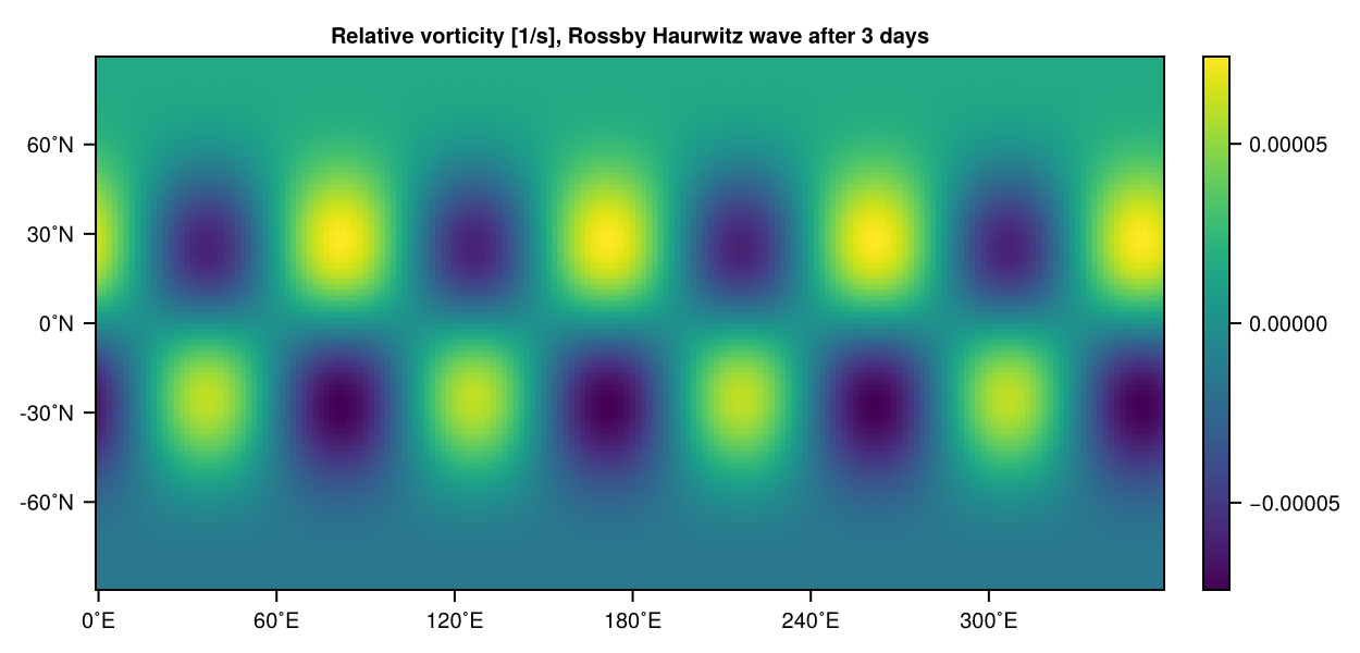

Looks like before, but shifted eastward! That's the Rossby-Haurwitz wave. The set! function accepts not just a function as outlined above, but also scalars, like set!(simulation, div=0) (which is always the case in the BarotropicModel) or grids, or LowerTriangularArrays representing variables in the spectral space. See ?set!, the set! docstring for more details.

Rossby-Haurwitz wave in a ShallowWater model

For the shallow water model also give initial conditions for the prognostic variable height    (equivalent to geopotential). The layer thickness is and is the interface displacement of that layer. SpeedyWeather however, uses as prognostic variable for which the initial conditions are

Where is the radius of the planet on which we consider the Rossby-Haurwitz wave, this value can be found in model.planet.radius and and are the rotation and the gravity constant of the planet, which are in model.planet.rotation and model.planet.gravity.

The interface displacement in SpeedyWeather's ShallowWaterModel is stored in the variable pres in analogy to the actual pressure in the primitive equation model. So we can set using set!(simulation, pres=η) for an appropriate implementation of the above equations, similar to how ζ(λ, θ, σ) = is defined above. However, we also already defined RossbyHaurwitzWave to do exactly that. With the following we can do a test run of the Rossby-Haurwitz wave in the shallow water model without any influences from orography.

spectral_grid = SpectralGrid(truncation=64, nlayers=1)
initial_conditions = RossbyHaurwitzWave(spectral_grid)
orography = NoOrography(spectral_grid)
forcing = nothing
drag = nothing
model = ShallowWaterModel(spectral_grid; forcing, drag, initial_conditions, orography)
simulation = initialize!(model)
run!(simulation, period=Day(8))

vor = get_step(simulation.variables.grid.vorticity)[:, 1]
heatmap(vor, title="Relative vorticity [1/s], shallow water Rossby Haurwitz wave after 8 days")

There is a noticeable difference from the result in the barotropic model, where the wave moves around the globe keeping its shape. Here, it deforms around the poles and the vorticity patches develop an internal structure.

Rossby-Haurwitz wave in primitive equations

You can use set! or the predefined RossbyHaurwitzWave also in other models. For the BarotropicModel or the PrimitiveDryModel (or Wet) the definition for is skipped. The barotropic model does not have a pressure variable, the primitive equation model uses the logarithm of surface pressure, which is incompatible with being defined as an interface displacement. So here, the RossbyHaurwitzWave only includes relative vorticity in the initial conditions.

The following shows how you can use RossbyHaurwitzWave in a PrimitiveDryModel (or Wet) but you probably also want to set initial conditions for temperature and pressure to not start at zero Kelvin and zero pressure. Also no orography, and let's switch off all physics parameterizations with dynamics_only=true.

spectral_grid = SpectralGrid(truncation=43, nlayers=8)
initial_conditions = (;
                        vordiv=RossbyHaurwitzWave(spectral_grid),
                        temp=JablonowskiTemperature(spectral_grid),
                        pres=PressureOnOrography(spectral_grid))

orography = NoOrography(spectral_grid)
time_stepping = Leapfrog(spectral_grid, Δt_at_T32=Minute(30))   # 30min timestep scaled linearly

forcing = nothing
drag = nothing

model = PrimitiveDryModel(spectral_grid; time_stepping, initial_conditions, orography, forcing, drag, dynamics_only=true)
simulation = initialize!(model)
run!(simulation, period=Day(5))

Note that we chose a lower resolution here (T43) as we are simulating 8 vertical layers now too. Let us visualise the surface vorticity ([:, 8] is the lowermost layer)

vor = get_step(simulation.variables.grid.vorticity)[:, 8]
heatmap(vor, title="Relative vorticity [1/s], primitive Rossby-Haurwitz wave")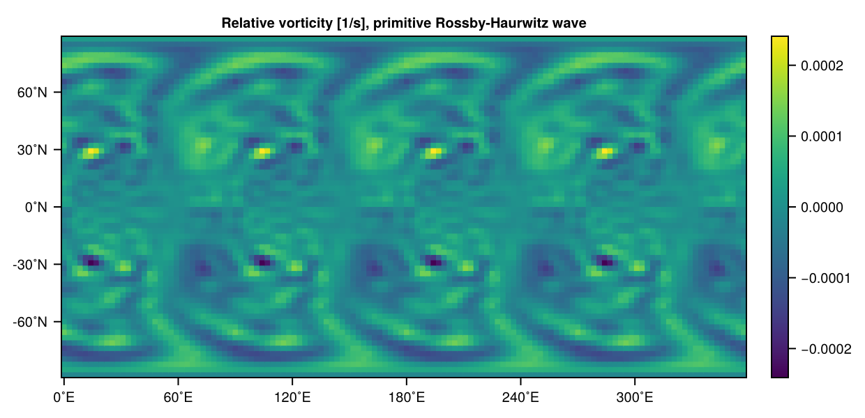

As you can see the actual Rossby-Haurwitz wave is not as stable any more (because those initial conditions are not a stable solution of the primitive equations) and so the 3-day integration looks already different from the barotropic model!

Default initial conditions for the PrimitiveWetModel

The PrimitiveWetModel starts by default from a state close to its own equilibrium climate, so that the model does not first have to adjust towards it. This matters mostly for humidity: a warm and moist tropical lower troposphere that is conditionally unstable would be rained out by the convection scheme within the first day.

using SpeedyWeather
spectral_grid = SpectralGrid(truncation = 32, nlayers = 8)
InitialConditions(spectral_grid, PrimitiveWet)

(zonal = BalancedZonalState{Float32} <: SpeedyWeather.AbstractInitialConditions
├ u₀::Float32 = 56.0
├ H::Float32 = 2.0
├ σ_jet::Float32 = 0.3
├ jet_decay::Float32 = 1.5
├ Tmin::Float32 = 226.0
├ perturb_lat::Float32 = 40.0
├ perturb_lon::Float32 = 20.0
├ perturb_uₚ::Float32 = 1.0
└ perturb_radius::Float32 = 0.1, humid = ConstantRelativeHumidity{Float32} <: SpeedyWeather.AbstractInitialConditions
├ relhumid_ref::Float32 = 0.7
├ σ_moist::Float32 = 0.25
└ σ_dry::Float32 = 0.1)

BalancedZonalState sets vorticity, divergence, surface pressure and temperature. It generalises the Jablonowski-Williamson initial conditions () to a different vertical profile of the zonal wind . With the dimensionless log-pressure coordinate    (zero at the surface, increasing upwards, but not a height in meters),

which is zero at the surface and increases about linearly with in the troposphere. Above    the wind decays with

so that the jet peaks in the upper troposphere (about   for the defaults σ_jet = 0.3 and jet_decay = D = 1.5) and not at the model top. The decaying wind requires, through thermal wind balance, a reversed meridional temperature gradient above the jet, i.e. a polar lower stratosphere that is warmer than the tropical one, as observed and as in . With the defaults the poles are up to about 40K warmer at  , which is more than in the real atmosphere. The initial conditions are still balanced, but whether the model's radiation maintains this stratosphere is a different question, so the jet may drift up or down over time. Use σ_jet = 0 for  , i.e. a wind that increases monotonically up to the model top with the poles colder than the tropics at all heights. That is closer to the equilibrium climate of the PrimitiveWetModel at the moment, which lacks the stratospheric warming at the poles, e.g. from ozone. Thermal wind balance then determines the temperature

with      and    , radius and rotation . Jablonowski and Williamson's temperature is the special case  . and have a zero global mean, so   is the global-mean temperature and can be chosen freely without breaking the balance. As in Jablonowski-Williamson a small perturbation of the zonal wind triggers baroclinic instability.

Derivation

The temperature follows from the same balance that Jablonowski and Williamson use, only without fixing the vertical profile of the wind. With a uniform surface pressure the gradient-wind balance on the sphere is

with   and geopotential . Differentiating with respect to and using hydrostatic balance   gives the thermal wind equation in its gradient-wind form

Inserting   the right-hand side separates into times two functions of latitude, (Coriolis term) and (curvature term). These are exactly and  , so integrating in latitude yields the temperature above. The integration constants in and ( and ) are chosen such that both have zero global mean, which leaves the global-mean temperature as a free function of height that does not affect the balance. The vorticity is the curl of , i.e. Jablonowski and Williamson's eq. (3) with in place of , and the divergence is zero apart from the perturbation.

This is not the moist baroclinic wave of the DCMIP-2016 intercomparison (), which prescribes a different analytic temperature (and a specific humidity profile) chosen for a reproducible test case, not to be close to a given model's climate. The point here is that only and are free, and they can be shaped like the model's climate while the balance is guaranteed analytically.

Parameters

The surface temperature and the lapse rate are taken from the atmosphere, model.atmosphere.reference_temperature and SpeedyWeather.lapse_rate(model.atmosphere) (the moist_lapse_rate for wet atmospheres, the dry_lapse_rate for dry ones), so that the initial conditions start from the climate the atmosphere is meant to have. Change them there, e.g. EarthAtmosphere(spectral_grid, reference_temperature = 283), which also changes other components that use these reference values. The remaining parameters were chosen to be close to the equilibrium climate of the default PrimitiveWetModel, by comparing against zonal and time means over days 60-120 of a long run at T32L8, T64L8 and T32L16 (which agree within about 2K). No formal optimisation was done; the parameters were read off these means:

Parameter	Default	How it was chosen
	288 K	atmosphere.reference_temperature
	5.7 K/km	atmosphere.moist_lapse_rate, slope of the global-mean against in the troposphere, which is
	226 K	Roughly isothermal global-mean stratosphere
	56 m/s	Zonal-mean wind at 45°, about 40 m/s at
	2	Wind growing about linearly in through the troposphere
	0.3	Jet at about  , as in observations and
	1.5	Weak wind at the model top while keeping the reversed temperature gradient moderate

With and fixed by the wind, the meridional temperature contrast (about 45K equator to pole near the surface) is no longer free but follows from the balance, and it agrees with the equilibrium to a few Kelvin. These parameters therefore describe the climate of a specific version of SpeedyWeather with its default parameterizations. If you change the physics, resolution or the planet substantially, the model's climate will change and to start close to the new equilibrium the parameters need to be adapted the same way: run the model into equilibrium (a few months), compute the zonal and time-mean temperature and zonal wind, fit (of the atmosphere) to the global-mean temperature profile, to the stratosphere and to the wind at mid-latitudes, then check that the resulting meridional temperature contrast is reasonable. The initial conditions remain balanced for any choice of parameters, only how close they are to the equilibrium climate depends on them.

Over orography the surface pressure is set hydrostatically with the temperature   at orographic height (in meters) and the temperature above is evaluated with   in place of . Air over a mountain is then as cold as the free atmosphere at the same pressure, otherwise the initial imbalance between surface pressure and temperature radiates gravity waves. BalancedZonalState therefore should not be combined with PressureOnOrography, which would overwrite its surface pressure.

ConstantRelativeHumidity then sets the humidity to a relative humidity of relhumid_ref below σ_moist, decreasing linearly to zero at σ_dry for a dry stratosphere. Use σ_moist = σ_dry = 0 for a vertically constant relative humidity instead.

To change these, pass a new NamedTuple of initial conditions, e.g. a weaker jet, or the Jablonowski-Williamson initial conditions

initial_conditions = (;
    zonal = BalancedZonalState(spectral_grid, u₀ = 40),
    humid = ConstantRelativeHumidity(spectral_grid, relhumid_ref = 0.6),
)

# or
initial_conditions = (;
    vordiv = ZonalWind(spectral_grid),
    temp = JablonowskiTemperature(spectral_grid),
    pres = PressureOnOrography(spectral_grid),
    humid = ConstantRelativeHumidity(spectral_grid),
)
model = PrimitiveWetModel(spectral_grid; initial_conditions)

Humidity is computed from temperature and pressure, so it has to come last in the NamedTuple.