Land surface model
The land surface in SpeedyWeather is represented through several components each of which can be changed in a modular way.
The actual LandModel or DryLandModel describing the equations for soil temperature and soil moisture, and vegetation or rivers.
The surface Albedo
The Orography
As these components are largely independent of another, it is possible to have a white (albedo high) ocean at the top of Mt Everest, or to paint the Sahara black and moving it below sea-level. The first one of these bullet points is discussed below for the others see the respective sections.
It's also possible to use a land model from Terrarium.jl within SpeedyWeather.jl. This is particularly relevant for higher complexity climate simulations as Terrarium features many more processes as our own build-in land models, see Terrarium coupling.
Dry vs wet land
The type hierarchy of theactual land surface model is defined as
using SpeedyWeather
subtypes(SpeedyWeather.AbstractLand)
2-element Vector{Any}:
SpeedyWeather.AbstractDryLand
SpeedyWeather.AbstractWetLandSo that a dry land does not have moisture whether the atmosphere is a PrimitiveWetModel (with humidity so it can rain) or a PrimitiveDryModel (without humidity). In contrast a wet land does have some soil moisture (which can be zero) and in combination with a PrimitiveWetModel will increase with precipitation for example. You can combine dry and wet land and dry and wet atmosphere freely.
LandModel
The default LandModel in SpeedyWeather contains (at the moment other than 2 soil layers are not supported or experimental)
spectral_grid = SpectralGrid(trunc=31, nlayers=8)
geometry = LandGeometry(spectral_grid, nlayers=2) # that's also the default, therefore it's optional here
land = LandModel(spectral_grid; geometry)LandModel{LandGeometry{Vector{Float32},...} <: SpeedyWeather.AbstractWetLand
├ spectral_grid::SpectralGrid{CPU{KernelAbstractions.CPU}, Spectrum{CPU{Kerne...
├ geometry::LandGeometry{Vector{Float32}, Int64}
├ thermodynamics::LandThermodynamics{Float32}
├ temperature::LandBucketTemperature{Float32}
├ soil_moisture::LandBucketMoisture{Float32}
├ snow::SnowModel{Float32}
├ vegetation::VegetationClimatology{Float32, Field{Float32, 1, Vector{Float32...
└ rivers::NothingWith LandGeometry currently used to define the number of soil layers and their layer thickness
land.geometryLandGeometry{Vector{Float32}, Int64} <: SpeedyWeather.AbstractLandGeometry
├ nlayers::Int64 = 2
└ arrays: layer_thicknessAnd land.thermodynamics used to define thermodynamics-relevant surface properties as conceptual "constants" used in the other components of the land surface model land.
land.thermodynamicsLandThermodynamics{Float32} <: SpeedyWeather.AbstractLandThermodynamics
├ heat_conductivity_dry_soil::Float32 = 0.42
├ heat_conductivity_snow::Float32 = 0.08
├ field_capacity::Float32 = 0.3
├ heat_capacity_water::Float32 = 4.2e6
├ heat_capacity_snow::Float32 = 2090.0
├ heat_capacity_dry_soil::Float32 = 1.13e6
├ soil_density::Float32 = 1700.0
└ wilting_point::Float32 = 0.17To change these you can either mutate the fields or create a new model component thermodynamics passed on to the land model constructor
thermodynamics = LandThermodynamics(spectral_grid, heat_conductivity_dry_soil=0.25)
land = LandModel(spectral_grid; thermodynamics)
land.thermodynamicsLandThermodynamics{Float32} <: SpeedyWeather.AbstractLandThermodynamics
├ heat_conductivity_dry_soil::Float32 = 0.25
├ heat_conductivity_snow::Float32 = 0.08
├ field_capacity::Float32 = 0.3
├ heat_capacity_water::Float32 = 4.2e6
├ heat_capacity_snow::Float32 = 2090.0
├ heat_capacity_dry_soil::Float32 = 1.13e6
├ soil_density::Float32 = 1700.0
└ wilting_point::Float32 = 0.17(note that ; thermodynamics is a Julia shortcut instead of thermodynamics=thermodynamics we often use matching keyword arguments by their name). Similarly you can change land.geometry which however is not mutable.
Generally, a LandModel or DryLandModel is similarly constructed to a PrimitiveWetModel or PrimitiveDryModel. One starts by defining its non-default components, always passes on the spectral grid as the first argument, and then constructs the actual land model by passing on those components. Finally, we use that land model to construct the atmospheric model
model = PrimitiveWetModel(spectral_grid; land)
model.landLandModel{LandGeometry{Vector{Float32},...} <: SpeedyWeather.AbstractWetLand
├ spectral_grid::SpectralGrid{CPU{KernelAbstractions.CPU}, Spectrum{CPU{Kerne...
├ geometry::LandGeometry{Vector{Float32}, Int64}
├ thermodynamics::LandThermodynamics{Float32}
├ temperature::LandBucketTemperature{Float32}
├ soil_moisture::LandBucketMoisture{Float32}
├ snow::SnowModel{Float32}
├ vegetation::VegetationClimatology{Float32, Field{Float32, 1, Vector{Float32...
└ rivers::Nothingis now the land defined above used when integrating a SpeedyWeather model.
In case a non-default number of soil layers is used, the LandGeometry also needs to be passed to the NetCDFOutput constructor to allocate the correct dimensions of the output variables, when an output is desired:
output = NetCDFOutput("output.nc", model, land_geometry)DryLandModel
Alternatively, one can use the DryLandModel to explicitly disable any functionality around soil moisture. By doing so, soil moisture will always be zero, or treated like zero skipping unnecessary computations. It is created in the same way (reusing some non-default thermodynamics from above)
land = DryLandModel(spectral_grid; thermodynamics)DryLandModel{LandGeometry{Vector{Float32},...} <: SpeedyWeather.AbstractDryLand
├ spectral_grid::SpectralGrid{CPU{KernelAbstractions.CPU}, Spectrum{CPU{Kerne...
├ geometry::LandGeometry{Vector{Float32}, Int64}
├ thermodynamics::LandThermodynamics{Float32}
└ temperature::LandBucketTemperature{Float32}but it does not contain soil moisture, vegetation or rivers in contrast to the LandModel.
Land soil temperature
Currently implemented soil temperatures are
subtypes(SpeedyWeather.AbstractLandTemperature)3-element Vector{Any}:
ConstantLandTemperature
LandBucketTemperature
SeasonalLandTemperatureYou can use them by passing them on to a LandModel/DryLandModel model constructor
temperature = LandBucketTemperature(spectral_grid)
land = LandModel(spectral_grid; temperature)LandModel{LandGeometry{Vector{Float32},...} <: SpeedyWeather.AbstractWetLand
├ spectral_grid::SpectralGrid{CPU{KernelAbstractions.CPU}, Spectrum{CPU{Kerne...
├ geometry::LandGeometry{Vector{Float32}, Int64}
├ thermodynamics::LandThermodynamics{Float32}
├ temperature::LandBucketTemperature{Float32}
├ soil_moisture::LandBucketMoisture{Float32}
├ snow::SnowModel{Float32}
├ vegetation::VegetationClimatology{Float32, Field{Float32, 1, Vector{Float32...
└ rivers::Nothingsuch that
land.temperatureLandBucketTemperature{Float32} <: SpeedyWeather.AbstractLandTemperature
├ mask::Bool = true
└ ocean_temperature::Float32 = 285.0is the LandBucketTemperature just defined. Similarly
land = DryLandModel(spectral_grid; temperature)DryLandModel{LandGeometry{Vector{Float32},...} <: SpeedyWeather.AbstractDryLand
├ spectral_grid::SpectralGrid{CPU{KernelAbstractions.CPU}, Spectrum{CPU{Kerne...
├ geometry::LandGeometry{Vector{Float32}, Int64}
├ thermodynamics::LandThermodynamics{Float32}
└ temperature::LandBucketTemperature{Float32}if you do not want the land to hold any moisture, vegetation or rivers.
LandBucketTemperature
LandBucketTemperature is a prognostic model of the soil temperature in the land surface model, interacting two-way with the surface air temperature. It can warm up through radiation and other surface heat fluxes, retain thermal energy and release this back to the atmosphere either in the form of longwave radiative fluxes or sensible heat fluxes (latent heat fluxes depend on soil moisture, see Surface fluxes). It is a bucket model such that interaction between neighbouring grid cells ("buckets") of the land surface only interact through the atmosphere with another, there are no direct horizontal fluxes between cells. In the sense of soil moisture, you can fill a bucket from above with rainfall, it may leak/drain at the bottom but buckets are laterally isolated from another. A similar concept applies to the heat fluxes of the LandBucketTemperature.
The LandBucketTemperature here follows MITgcm's 2-layer model, as defined here. As this is a 2-layer model, SpectralGrid(nlayers_soil=2) is required. The equations are
for two layers of thicknesses F (in
The heat capacities
with
Land soil moisture
Currently implemented soil moistures are
subtypes(SpeedyWeather.AbstractSoilMoisture)2-element Vector{Any}:
LandBucketMoisture
SeasonalSoilMoistureYou can use them by passing them on to a LandModel (not the DryLandModel though which does not have moisture) model constructor
soil_moisture = LandBucketMoisture(spectral_grid)
land = LandModel(spectral_grid; soil_moisture)LandModel{LandGeometry{Vector{Float32},...} <: SpeedyWeather.AbstractWetLand
├ spectral_grid::SpectralGrid{CPU{KernelAbstractions.CPU}, Spectrum{CPU{Kerne...
├ geometry::LandGeometry{Vector{Float32}, Int64}
├ thermodynamics::LandThermodynamics{Float32}
├ temperature::LandBucketTemperature{Float32}
├ soil_moisture::LandBucketMoisture{Float32}
├ snow::SnowModel{Float32}
├ vegetation::VegetationClimatology{Float32, Field{Float32, 1, Vector{Float32...
└ rivers::NothingLandBucketMoisture
LandBucketMoisture defines the prognostic equation for soil moisture in the land surface model. It is a bucket model in the sense that every grid cell can fill like a bucket with rainfall from above dry out by evaporation, can drain into layers below or into a river runoff. But there is generally no lateral transport, only through the atmosphere.
The LandBucketMoisture here follows MITgcm's 2-layer model, as defined here. As this is a 2-layer model, SpectralGrid(nlayers_soil=2) is required. The equations are
for soil moistures
At the moment (and generally if not coupled to an ocean model) the river runoff lets water disappear.
Snow model
SpeedyWeather has a simple snow model that allows for snow to lie on land and impact albedo and isolate air-land fluxes. Snow is created from the precipitation schemes, can melt on the ground depending on soil temperature where it is then passed to the soil moisture. We also include a runoff/relaxation term to prevent snow piling up without bounds as soil temperatures below freezing would never remove such snow. In reality this is where one needs a ice sheet model to convert the snow to ice and simulate ice flow like in a glacier or in the Greenland and Antarctic ice sheets.
LandSnowModel
SnowModel stores a single snow bucket with depth variables.prognostic.land.snow_depth) and solves the following equation
with precipitation snow_rate (
The available melt energy in the top layer of thickness
This is the maximum melt rate
with
Snowfall and melt form a raw tendency
in excess term (negative for melting trying to remove more snow than there is) only appears when the naive tendency would overdraw the bucket. snow_melt_rate is zero over ocean points. Negative snow depth is clamped to zero (technically redundant given the conserving excess term above) and stored as equivalent liquid water height, not physical snow thickness. The accumulation is capped at 10m equivalent liquid water height, following how permanent snow area is treated in IFS Cycle 49r1. In reality very large accumulation of snow would form glaciers and eventually ice sheets that we do not simulate here.
The snow budget links into other surface schemes:
snow_melt_rateprovides a latent heat sink to the land temperature budget.The same flux (converted to
by dividing by ) feeds the soil moisture tendency alongside rain. Snow depth drives the snow-albedo calculation and insulates surface heat/humidity fluxes (see below).
Snow cover over land is diagnosed from snow depth using either a linear ramp
set via the snow_cover keyword of LandSnowAlbedo. Snow then adds an albedo to the land albedo (diagnosed from vegetation cover)
so snow depth from the snow bucket immediately brightens land grid cells. The total albedo is higher over already brighter areas (low vegetation cover) and lower over darker areas. This somewhat reflects that in forests the snow cover is broken up and snow lies in between trees.
Albedo
Albedo is the surface reflectivity to downward solar shortwave radiation. A value of 1 indicates that all of the radiative flux is reflected at the Earth's surface and sent back up through the atmospheric column. In contrast, a value of 0 means no reflection and all of that radiative flux is absorbed, typically heating ocean or land surface. The following albedo's are currently implemented
subtypes(SpeedyWeather.AbstractAlbedo)6-element Vector{Any}:
AlbedoClimatology
GlobalConstantAlbedo
LandSnowAlbedo
ManualAlbedo
OceanLandAlbedo
OceanSeaIceAlbedoAlbedo is generally a 2D global diagnostic variable for ocean and land separately. You can keep it constant or diagnose it from other fields on every time step: OceanSeaIceAlbedo mixes in sea ice concentration and LandSnowAlbedo uses the snow depth bucket described above. Conceptually albedo is not a static boundary condition but recomputed each step so transient surface changes (e.g. snowfall) brighten the surface without losing the underlying bare albedo. If you want to set albedo manually with set! then use ManualAlbedo which has its own albedo 2D field that is copied into the diagnostic variables on every time step. See example below. AlbedoClimatology does the same but ManualAlbedo does not need to read an albedo from file at initialization.
Albedo itself is a container for separate albedo's for ocean and land as averaging those in grid cells which are partially land, partially ocean will yield inaccurate results. Think 10% land having a lower heat capacity than land but being treated with an albedo that comes from 90% ocean. Not very realistic. The default albedo can be created with
albedo = OceanLandAlbedo(spectral_grid)OceanLandAlbedo{OceanSeaIceAlbedo{Float32}, L...} <: SpeedyWeather.AbstractAlbedo
├ ocean::OceanSeaIceAlbedo{Float32}
└ land::LandSnowAlbedo{Float32, SaturatingSnowCover}and inspected with
albedo.oceanOceanSeaIceAlbedo{Float32} <: SpeedyWeather.AbstractAlbedo
├ albedo_ocean::Float32 = 0.06
└ albedo_ice::Float32 = 0.6and albedo.land. You can mix those albedos too, they are internally two independent albedos that are applied to fluxes separately, e.g.
albedo = OceanLandAlbedo(GlobalConstantAlbedo(spectral_grid), AlbedoClimatology(spectral_grid))OceanLandAlbedo{GlobalConstantAlbedo{Float32}...} <: SpeedyWeather.AbstractAlbedo
├ ocean::GlobalConstantAlbedo{Float32}
└ land::AlbedoClimatology{Field{Float32, 1, Vector{Float32}, OctahedralGaussi...constructs an albedo that is a global constant (default 0.3) for the ocean but the AlbedoClimatology read from file used for the land. The first argument for Albedo is used for ocean the second for land but you can use keywords too.
Alternatively you can also drop the separation into ocean/land albedo (e.g. idealised simulations or aqua planet, rocky planet). And just use
albedo = GlobalConstantAlbedo(spectral_grid)GlobalConstantAlbedo{Float32} <: SpeedyWeather.AbstractAlbedo
└ albedo::Float32 = 0.3and this definition of the albedo will be used for both ocean and land fluxes. In all cases you can then pass on the albedo to the model constructor, e.g.
albedo = OceanLandAlbedo(GlobalConstantAlbedo(spectral_grid, albedo=0.1), ManualAlbedo(spectral_grid))
set!(albedo.land, (λ, φ) -> 0.2 + 0.3*abs(φ)/90)

model = PrimitiveWetModel(spectral_grid; albedo)
model.albedoOceanLandAlbedo{GlobalConstantAlbedo{Float32}...} <: SpeedyWeather.AbstractAlbedo
├ ocean::GlobalConstantAlbedo{Float32}
└ land::ManualAlbedo{Field{Float32, 1, Vector{Float32}, OctahedralGaussianGri...The albedo in the model is now the one defined just in the lines above, using a globally constant albedo of 0.1 for the ocean but a higher albedo over land which also increases to 0.5 towards the poles.
You can always output the land-sea mask weighted albedo with add!(model, SpeedyWeather.AlbedoOutput()) or inspect it as follows
simulation = initialize!(model)
run!(simulation, steps=1)   # run for a step to "diagnose" albedo = ocean/land weighted

using CairoMakie
(; albedo) = simulation.variables.parameterizations
heatmap(albedo, title="Custom albedo, separately defined for ocean/land")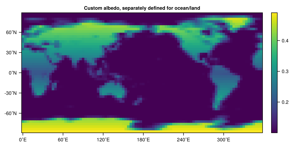
Terrarium coupling
We can also use a Terrarium model within SpeedyWeather! For a detailed introduction to Terrarium please consult its own documentation. Here, we will only demonstrate the coupling.
Example
We first have to construct our Terrarium model, before we can wrap it into a SpeedyWeather.LandModel and construct a PrimitiveWetModel with it:
using SpeedyWeather
using Terrarium

# SpeedyWeather grid + matching Terrarium column ring grid
ring_grid     = SpeedyWeather.RingGrids.FullGaussianGrid(12)
spectral_grid = SpectralGrid(ring_grid)

# load and sync the land sea mask for both SpeedyWeather and Terrarium
land_sea_mask = EarthLandSeaMask(spectral_grid)
SpeedyWeather.load_mask!(land_sea_mask)

Nz       = 4
Δz_min   = 0.05
column_grid = Terrarium.ColumnRingGrid(
    Terrarium.CPU(), Float32,
    Terrarium.ExponentialSpacing(; N = Nz, Δz_min),
    ring_grid,
    land_sea_mask,
)

# Soil column + initial state, matching `LandModel: Soil, no vegetation`
soil_initializer = Terrarium.SoilInitializer(eltype(column_grid))
soil = Terrarium.SoilEnergyWaterCarbon(
    eltype(column_grid);
    hydrology = Terrarium.SoilHydrology(eltype(column_grid)),
)
terrarium_model = Terrarium.LandModel(
    column_grid;
    initializer = soil_initializer,
    vegetation  = nothing,
    soil,
)

# Wrap as a SpeedyWeather land component (time step Δt = 300 s)
land = SpeedyWeather.LandModel(spectral_grid, terrarium_model; Δt = 300.0)

# Assemble the wet primitive model around `land`
model = PrimitiveWetModel(
    spectral_grid;
    land,
    land_sea_mask,
    surface_heat_flux     = SurfaceHeatFlux(spectral_grid, land = PrescribedLandHeatFlux()),
    surface_humidity_flux = SurfaceHumidityFlux(spectral_grid, land = PrescribedLandHumidityFlux()),
    time_stepping         = Leapfrog(spectral_grid, Δt_at_T31 = Minute(15)),
)

simulation = initialize!(model)Simulation{...} (2.26 MB)
├ variables::Variables{...} (1.88 MB)
└ model::PrimitiveWetModel{...} (409.07 KB)Then the model can be run as any other Simulation. Terarrium's state variales are owned by SpeedyWeather's Variables and can be accessed via
simulation.variables.prognostic.land.terrariumStateVariables{Float32}
├─ Clock: Clock{DateTime, Float64}(time=0000-12-31T00:00:00, iteration=0, last_Δt=Inf days)
├── stage: 1
└── last_stage_Δt: Inf days
├─ Prognostic: NamedTuple with 2 Fields on 611×1×4 RectilinearGrid{Float32, Periodic, Flat, Bounded} on CPU with 3×0×3 halo:
├── internal_energy: 611×1×4 Field{Oceananigans.Grids.Center, Oceananigans.Grids.Center, Oceananigans.Grids.Center} on Oceananigans.Grids.RectilinearGrid on CPU
└── skin_temperature: 611×1×1 Field{Oceananigans.Grids.Center, Oceananigans.Grids.Center, Nothing} reduced over dims = (3,) on Oceananigans.Grids.RectilinearGrid on CPU
├─ Auxiliary: NamedTuple with 17 Fields on 611×1×4 RectilinearGrid{Float32, Periodic, Flat, Bounded} on CPU with 3×0×3 halo:
├── temperature: 611×1×4 Field{Oceananigans.Grids.Center, Oceananigans.Grids.Center, Oceananigans.Grids.Center} on Oceananigans.Grids.RectilinearGrid on CPU
├── liquid_water_fraction: 611×1×4 Field{Oceananigans.Grids.Center, Oceananigans.Grids.Center, Oceananigans.Grids.Center} on Oceananigans.Grids.RectilinearGrid on CPU
├── ground_temperature: 611×1×1 Field{Oceananigans.Grids.Center, Oceananigans.Grids.Center, Oceananigans.Grids.Center} on Oceananigans.Grids.RectilinearGrid on CPU
├── saturation_water_ice: 611×1×4 Field{Oceananigans.Grids.Center, Oceananigans.Grids.Center, Oceananigans.Grids.Center} on Oceananigans.Grids.RectilinearGrid on CPU
├── water_table: 611×1×1 Field{Oceananigans.Grids.Center, Oceananigans.Grids.Center, Nothing} reduced over dims = (3,) on Oceananigans.Grids.RectilinearGrid on CPU
├── hydraulic_conductivity: 611×1×5 Field{Oceananigans.Grids.Center, Oceananigans.Grids.Center, Oceananigans.Grids.Face} on Oceananigans.Grids.RectilinearGrid on CPU
├── ground_heat_flux: 611×1×1 Field{Oceananigans.Grids.Center, Oceananigans.Grids.Center, Nothing} reduced over dims = (3,) on Oceananigans.Grids.RectilinearGrid on CPU
├── surface_shortwave_up: 611×1×1 Field{Oceananigans.Grids.Center, Oceananigans.Grids.Center, Nothing} reduced over dims = (3,) on Oceananigans.Grids.RectilinearGrid on CPU
├── surface_longwave_up: 611×1×1 Field{Oceananigans.Grids.Center, Oceananigans.Grids.Center, Nothing} reduced over dims = (3,) on Oceananigans.Grids.RectilinearGrid on CPU
├── surface_net_radiation: 611×1×1 Field{Oceananigans.Grids.Center, Oceananigans.Grids.Center, Nothing} reduced over dims = (3,) on Oceananigans.Grids.RectilinearGrid on CPU
├── sensible_heat_flux: 611×1×1 Field{Oceananigans.Grids.Center, Oceananigans.Grids.Center, Nothing} reduced over dims = (3,) on Oceananigans.Grids.RectilinearGrid on CPU
├── latent_heat_flux: 611×1×1 Field{Oceananigans.Grids.Center, Oceananigans.Grids.Center, Nothing} reduced over dims = (3,) on Oceananigans.Grids.RectilinearGrid on CPU
├── rainfall_ground: 611×1×1 Field{Oceananigans.Grids.Center, Oceananigans.Grids.Center, Nothing} reduced over dims = (3,) on Oceananigans.Grids.RectilinearGrid on CPU
├── ground_evaporation_conductance: 611×1×1 Field{Oceananigans.Grids.Center, Oceananigans.Grids.Center, Nothing} reduced over dims = (3,) on Oceananigans.Grids.RectilinearGrid on CPU
├── evaporation_ground: 611×1×1 Field{Oceananigans.Grids.Center, Oceananigans.Grids.Center, Nothing} reduced over dims = (3,) on Oceananigans.Grids.RectilinearGrid on CPU
├── surface_runoff: 611×1×1 Field{Oceananigans.Grids.Center, Oceananigans.Grids.Center, Nothing} reduced over dims = (3,) on Oceananigans.Grids.RectilinearGrid on CPU
└── infiltration: 611×1×1 Field{Oceananigans.Grids.Center, Oceananigans.Grids.Center, Nothing} reduced over dims = (3,) on Oceananigans.Grids.RectilinearGrid on CPU
├─ Inputs: NamedTuple with 10 Fields on 611×1×4 RectilinearGrid{Float32, Periodic, Flat, Bounded} on CPU with 3×0×3 halo:
├── air_temperature: 611×1×1 Field{Oceananigans.Grids.Center, Oceananigans.Grids.Center, Nothing} reduced over dims = (3,) on Oceananigans.Grids.RectilinearGrid on CPU
├── air_pressure: 611×1×1 Field{Oceananigans.Grids.Center, Oceananigans.Grids.Center, Nothing} reduced over dims = (3,) on Oceananigans.Grids.RectilinearGrid on CPU
├── windspeed: 611×1×1 Field{Oceananigans.Grids.Center, Oceananigans.Grids.Center, Nothing} reduced over dims = (3,) on Oceananigans.Grids.RectilinearGrid on CPU
├── specific_humidity: 611×1×1 Field{Oceananigans.Grids.Center, Oceananigans.Grids.Center, Nothing} reduced over dims = (3,) on Oceananigans.Grids.RectilinearGrid on CPU
├── rainfall: 611×1×1 Field{Oceananigans.Grids.Center, Oceananigans.Grids.Center, Nothing} reduced over dims = (3,) on Oceananigans.Grids.RectilinearGrid on CPU
├── snowfall: 611×1×1 Field{Oceananigans.Grids.Center, Oceananigans.Grids.Center, Nothing} reduced over dims = (3,) on Oceananigans.Grids.RectilinearGrid on CPU
├── surface_shortwave_down: 611×1×1 Field{Oceananigans.Grids.Center, Oceananigans.Grids.Center, Nothing} reduced over dims = (3,) on Oceananigans.Grids.RectilinearGrid on CPU
├── surface_longwave_down: 611×1×1 Field{Oceananigans.Grids.Center, Oceananigans.Grids.Center, Nothing} reduced over dims = (3,) on Oceananigans.Grids.RectilinearGrid on CPU
├── daytime_length: 611×1×1 Field{Oceananigans.Grids.Center, Oceananigans.Grids.Center, Nothing} reduced over dims = (3,) on Oceananigans.Grids.RectilinearGrid on CPU
└── CO2: 611×1×1 Field{Oceananigans.Grids.Center, Oceananigans.Grids.Center, Nothing} reduced over dims = (3,) on Oceananigans.Grids.RectilinearGrid on CPU
├─ Namespaces: (:soil,)
└─ Timestepper cache: ()Output of Terrarium variables
Any variable of the Terrarium state (prognostic, auxiliary/diagnostic, or input) can be written to SpeedyWeather's output with TerrariumOutput. Its name, units, long name and dimensionality are derived automatically from Terrarium's variable metadata. Add all prognostic and auxiliary Terrarium variables with
add!(model, TerrariumOutput(terrarium_model)...)NetCDFOutput{Field{Float32, 1, Vector{Floa...}
├ status: inactive/uninitialized
├ write restart file = true (if active)
├ interpolator::AnvilInterpolator{Float32, GridGeometry{FullGaussianGrid{CPU{KernelAbs...}
├ path = output.nc (overwrite=false)
├ interval = 21600 seconds
└ variables
├ surface_longwave_up: Outgoing (upwelling) longwave radiation [W m^-2]
├ ground_temperature: Temperature of the uppermost ground or soil grid cell in °C [°C]
├ rainfall_ground: Rainfall rate reaching the ground [m s^-1]
├ skin_temperature: Longwave emission temperature of the land surface in °C [°C]
├ temperature: Temperature of the soil volume in °C [°C]
├ water_table: Elevation of the water table in meters [m]
├ sensible_heat_flux: Sensible heat flux at the surface [W m⁻²] [W m^-2]
├ liquid_water_fraction: Fraction of unfrozen water in the pore space [1]
├ infiltration: Infiltration flux [m s^-1]
├ temp: temperature [degC]
├ surface_runoff: Total surface runoff [m s^-1]
├ evaporation_ground: Ground evaporation contribution to surface humidity flux [m s^-1]
├ mslp: mean sea-level pressure [hPa]
├ vor: relative vorticity [s^-1]
├ surface_shortwave_up: Outgoing (upwelling) shortwave radiation [W m^-2]
├ v: meridional wind [m/s]
├ u: zonal wind [m/s]
├ ground_evaporation_conductance: Ground evaporation vapor conductance [m s^-1]
├ internal_energy: Internal energy of the soil volume, including both latent and sensible components [J m^-3]
├ latent_heat_flux: Latent heat flux at the surface [W m⁻²] [W m^-2]
├ humid: specific humidity [kg/kg]
├ saturation_water_ice: Saturation level of water and ice in the pore space [1]
├ ground_heat_flux: Ground heat flux [W m^-2]
└ surface_net_radiation: Net radiation budget [W m^-2]or add a single variable (here renamed in the output file via name, any Terrarium variable name works, e.g. also :saturation_water_ice or :sensible_heat_flux) with
add!(model, TerrariumOutput(terrarium_model, :temperature, name = "soil_temperature"))Then run the simulation with run!(simulation, output = true) as usual. 3D (subsurface) variables like the soil temperature are written on an additional vertical dimension soil_depth with the depths of the Terrarium soil layer centres (in meters, positive down) as coordinates. Ocean grid points, where Terrarium does not simulate anything, are filled with NaN. Terrarium output variables are supported both with NetCDFOutput and, once Zarr.jl is loaded, with ZarrOutput:
using Zarr
output = ZarrOutput(spectral_grid, PrimitiveWet)
model = PrimitiveWetModel(spectral_grid; land, output, ...)
add!(model, TerrariumOutput(terrarium_model)...)