RingGrids
RingGrids is a package that has been developed for SpeedyWeather.jl and is used by it but can also be used standalone.
RingGrids defines several iso-latitude grids, which are mathematically described in the section on Grids. In brief, they include the regular latitude-longitude grids (here called FullClenshawGrid) as well as grids which latitudes are shifted to the Gaussian latitudes and reduced grids, meaning that they have a decreasing number of longitudinal points towards the poles to be more equal-area than full grids.
Defined grids
RingGrids defines and exports the following grids, see also Implemented grids for a more mathematical description.
Full grids
using RingGrids
subtypes(RingGrids.AbstractFullGrid)
4-element Vector{Any}:
FullClenshawGrid
FullGaussianGrid
FullHEALPixGrid
FullOctaHEALPixGridand reduced grids
subtypes(RingGrids.AbstractReducedGrid)5-element Vector{Any}:
HEALPixGrid
OctaHEALPixGrid
OctahedralClenshawGrid
OctahedralGaussianGrid
OctaminimalGaussianGridThe following explanation of how to use these can be mostly applied to any of them, however, there are certain functions that are not defined, e.g. the full grids can be trivially converted to a Matrix (i.e. they are rectangular grids) but not the OctahedralGaussianGrid.
What is a ring?
We use the term ring, short for iso-latitude ring, to refer to a sequence of grid points that all share the same latitude. A latitude-longitude grid is a ring grid, as it organises its grid-points into rings. However, other grids, like the cubed-sphere are not based on iso-latitude rings. SpeedyWeather.jl only works with ring grids because its a requirement for the Spherical Harmonic Transform to be efficient. See Grids.
Grid versus Field
With "grid" we mean the discretization of space. Also called tesselation given that we are tiling a space with polygons, we subdivide the sphere into grid cells, with vertices, faces and centres. In that sense, a grid does not contain any data it purely describes the location of grid cells. Grids in RingGrids are identified by their name, e.g. FullGaussianGrid, and a resolution parameter where we use nlat_half (the number of latitudes on one hemisphere, Equator included) for all grids. This is because some grids have an even number some an odd number number of latitudes so not all nlat are valid, but all nlat_half are. While an instance of a grid stores some precomputed arrays to facilitate faster indexing it does not store coordinates and similar grid information, these can be recomputed on the fly whenever needed given a grid. All grids are considered to be two-dimensional, so they do not contain information about the vertical or time, for example. The horizontal grid points are unravelled into a vector, starting at 0˚E at the north pole, going first east, then ring by ring to the south pole.
Data on a grid is called a Field, many variables, like temperature are a field. Surface temperature would be a 2D field (though represented as a vector), temperature on several vertical layers of the atmosphere would be 3D (data represented as a matrix, horizontal x vertical), including time would make it 4D. Several fields can share the same grid. Given that the grid is always two-dimensional, a 2D and 3D field can also share the same grid, leaving the 3rd dimension not further specified for flexibility.
Creating a grid
All grids are specified by name and the resolution parameter nlat_half::Integer (number of latitude rings on one hemisphere, Equator included). An instance of a grid is simply created by
grid = FullGaussianGrid(24)48-ring FullGaussianGrid{...}
├ nlat_half = 24 (4608 points, ~2.99˚, full)
└ architecture = CPUAs a second argument architecture can be provided which helps to share information on the computing architecture (CPU/GPU) but this will not be further explained here.
Accessing coordinates
With a grid you can get the coordinates through get_lat, get_latd, get_colat, get_lond but note that the latter is only defined for full grids as the reduced grids do not share the same longitudes across rings. To obtain the longitudes and latitudes for all grid points use get_londlatds, get_lonlats, get_loncolats, e.g.
grid = OctaminimalGaussianGrid(2)   # a tiny grid with 4 latitudes only
get_latd(grid)
4-element Vector{Float64}:
59.44440828916677
19.875719147440904
-19.875719147440904
-59.44440828916677Creating a Field
Creating Field, that means data on a grid can be done in many ways, for example using zeros, ones,rand, orrandn`
grid = HEALPixGrid(2)               # smallest HEALPix
field = zeros(grid)                 # 2D field
field = rand(grid, 10)              # 3D field with 10 vertical layers or time steps
field = randn(Float32, grid, 2, 2)  # 4D using Float32 as element type
12×2×2, 3-ring (XY+) HEALPixField{Float32, 3} as Array on CPU
[:, :, 1] =
-1.602102f0 1.0092921f0
-1.5539061f0 0.16345626f0
1.7261918f0 1.7849507f0
1.1297747f0 0.735487f0
0.36913058f0 -0.48859143f0
-1.9414517f0 -2.0755026f0
1.8397624f0 -1.2647109f0
-0.3803897f0 0.32168975f0
-1.530793f0 -0.3799753f0
-0.5935101f0 0.290133f0
-0.0041100057f0 0.15059522f0
0.759992f0 -0.91579217f0
[:, :, 2] =
0.4504584f0 1.7619836f0
0.7437716f0 0.2940806f0
0.5416388f0 0.41809902f0
-1.3349504f0 -1.4876962f0
-0.7697006f0 0.89928776f0
-1.0673361f0 0.27010262f0
-0.6544871f0 0.45600298f0
-0.31528565f0 2.3482528f0
1.5713271f0 2.1282694f0
-0.015803456f0 -0.66412085f0
0.5277684f0 -0.6278597f0
0.10514956f0 0.528475f0Note that in this case all fields share the same grid. Or the grid can be created on the fly when the grid type is specified, followed by nlat_half. Every ?Grid also has a corresponding ?Field type, e.g.
field = zeros(OctaminimalGaussianGrid, 2)   # nlat_half=2
field = HEALPixField(undef, 2)              # using undef initializor
field = HEALPixField{Float16}(undef, 2, 3)  # using Float16 as eltype
12×3, 3-ring (XY+) HEALPixField{Float16, 2} as Array on CPU
Float16(6.0e-8) Float16(2.0e-7) Float16(2.2e-6)
Float16(0.0) Float16(0.0) Float16(0.0)
Float16(0.0) Float16(0.0) Float16(0.0)
Float16(0.0) Float16(0.0) Float16(0.0)
Float16(0.0) Float16(6.0e-8) Float16(8.3e-7)
Float16(0.0) Float16(0.0) Float16(0.0)
Float16(0.0) Float16(0.0) Float16(0.0)
Float16(0.0) Float16(0.0) Float16(0.0)
Float16(6.0e-8) Float16(6.0e-8) NaN16
Float16(0.0) Float16(0.0) NaN16
Float16(0.0) Float16(0.0) NaN16
Float16(0.0) Float16(0.0) NaN16Array dimensions of a Field
Besides data and grid, a Field also carries a dims::AbstractArrayDimensions that records what the dimensions beyond the horizontal actually represent, e.g. vertical layers or time steps, see Array dimensions for a general overview of these dimension tags. The tags defined for Field are XY (2D, horizontal only, the default), XYZ (horizontal + vertical), XYT (horizontal + time), and XYZT (horizontal + vertical + time). They are bookkeeping only (they do not change how the field is indexed or computed on) but allow ArrayDimensions.hasvertical(field) and ArrayDimensions.hastime(field) to answer what a given non-horizontal dimension stands for, and they are preserved through similar, zero, views and indexing (dropping a dimension whenever you index into it with an integer).
To create a Field with an explicit dimension, pass an instance of one of these types as an extra argument, e.g. after the grid
grid = FullGaussianGrid(4)
field = zeros(grid, ArrayDimensions.XYZ(), 3)  # 3 layers are vertical, not time
ArrayDimensions.hasvertical(field), ArrayDimensions.hastime(field)
(true, false)If no dims is provided (as in Creating a Field) XY is used by default, meaning that no assumption is made about the meaning of any additional dimension.
Creating a Field from data
A field has field.data (some AbstractArray{T, N}) and field.grid (some AbstractGrid as described above). The first dimension of data describes the horizontal as the grid points on every grid (full and reduced) are unravelled west to east then north to south, meaning that it starts at 90˚N and 0˚E then walks eastward for 360˚ before jumping on the next latitude ring further south, this way circling around the sphere till reaching the south pole. This may also be called ring order.
Data in a Matrix which follows this ring order can be put on a FullGaussianGrid like so
data = randn(Float32, 8, 4)
field = FullGaussianGrid(data, input_as=Matrix)
field = FullGaussianField(data, input_as=Matrix)    # equivalent
32-element, 4-ring (XY) FullGaussianField{Float32, 1} as Array on CPU
-0.85405797f0
0.39508164f0
-1.7245182f0
-0.58374125f0
-1.6307176f0
0.74492705f0
-0.6752162f0
0.63019264f0
0.682746f0
-0.040053498f0
⋮
-0.63599426f0
-0.23119274f0
0.5772145f0
-0.9439476f0
-0.74111766f0
-1.128258f0
-0.9694421f0
-0.8833953f0
-1.595097f0Both return a field (there is no data in the grid itself) and create an instance of FullGaussianGrid on the fly. The input_as=Matrix is required to denote that the horizontal dimension is not unravelled into a vector, triggering a reshape internally, input_as=Vector is the default. A full Gaussian grid has always FullClenshawGrid has
If you have the data and know which grid it comes one you can also create a Field by providing both
data = randn(Float32, 8, 4)         # data of some shape
grid = OctaminimalGaussianGrid(1)   # you need to know the nlat_half (here 1) of that grid!
field = Field(data, grid)
8×4, 2-ring (XY+) OctaminimalGaussianField{Float32, 2} as Array on CPU
2.2901175f0 1.1842991f0 1.110093f0 -2.0924342f0
-0.05123722f0 -0.016481666f0 0.983656f0 -1.5804783f0
1.2581186f0 1.7863929f0 1.5693024f0 0.5397475f0
-0.23263851f0 0.4034763f0 -0.27387062f0 -0.7097382f0
-1.4521917f0 -0.5939481f0 0.31491715f0 0.08882695f0
0.7163305f0 -0.2581346f0 1.5633657f0 0.8434712f0
-0.3826157f0 -0.7159602f0 -0.4073266f0 1.2249746f0
-1.6434748f0 -1.2984451f0 0.9958369f0 -0.6474499f0But you can also automatically let nlat_half be calculated from the shape of the data. Note that you have to provide the name of the field though, FullGaussianField here to create a Field on a FullGaussianGrid.
field = FullGaussianField(data, input_as=Matrix)32-element, 4-ring (XY) FullGaussianField{Float32, 1} as Array on CPU
2.2901175f0
-0.05123722f0
1.2581186f0
-0.23263851f0
-1.4521917f0
0.7163305f0
-0.3826157f0
-1.6434748f0
1.1842991f0
-0.016481666f0
⋮
0.9958369f0
-2.0924342f0
-1.5804783f0
0.5397475f0
-0.7097382f0
0.08882695f0
0.8434712f0
1.2249746f0
-0.6474499f0To return to the original data array you can reshape the data of a full grid (which is representable as a matrix) as follows
data == Matrix(FullGaussianField(data, input_as=Matrix))truewhich in general is Array(field, as=Vector) for no reshaping (equivalent to field.data including possible conversion to Array) and Array(field, as=Matrix) with reshaping (full grids only).
Visualising Fields
As only the full fields can be reshaped into a matrix, the underlying data structure of any AbstractField is a vector for consistency. As shown in the examples above, one can therefore inspect the data as if it was a vector. But a field has through field.grid all the geometric information available to plot it on a map, SpeedyWeather also implements extensions for Makie's and UnicodePlots's' heatmap, also see Visualisation via Makie and Visualisation via UnicodePlots.
import CairoMakie: heatmap   # triggers loading of Makie extension, or use UnicodePlots instead!
grid = OctahedralGaussianGrid(24)
field = randn(grid)
heatmap(field)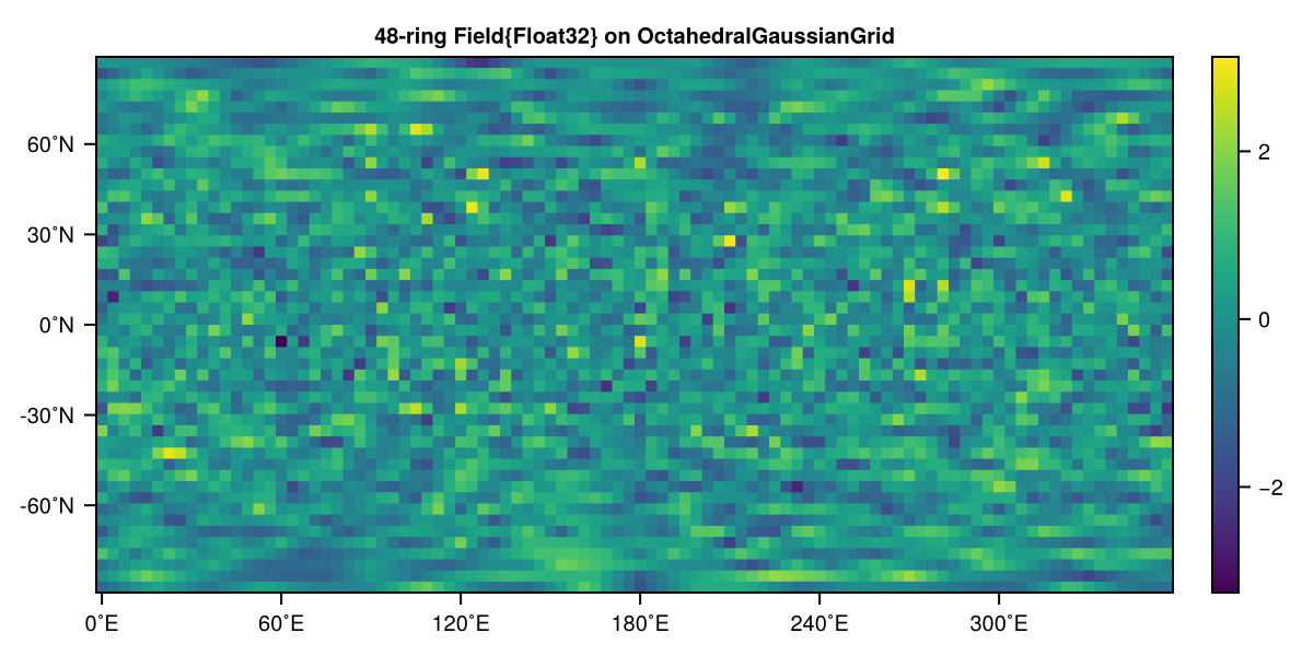
Reduced fields are automatically interpolated to the corresponding full fields so that they can be visualised as a matrix.
Indexing Fields
All fields have a single index ij which follows the ring order. While this is obviously not super exciting here are some examples how to make better use of the information that the data sits on a two-dimensional grid covering the sphere. We obtain the latitudes of the rings of a grid by calling get_latd (get_lond is only defined for full grids, or use get_londlatds for latitudes, longitudes per grid point not per ring). Now we could calculate Coriolis and add it on the grid as follows
grid = OctahedralClenshawGrid(5)    # define a grid
field = randn(grid)                 # random data on that grid
latd = get_latd(grid)               # get a vector of latitudes [˚N] per ring, north to south

rotation = 7.29e-5                  # angular frequency of Earth's rotation [rad/s]
coriolis = 2rotation*sind.(latd)    # vector of coriolis parameters per latitude ring

for (j, ring) in enumerate(eachring(field))     # loop over every ring j
    f = coriolis[j]
    for ij in ring                              # loop over every longitude point on that ring
        field[ij] += f
    end
end
eachring(field) accesses field.grid.rings a precomputed vector of UnitRange indices, such that we can loop over the ring index j (j=1 being closest to the North pole) pull the coriolis parameter at that latitude and then loop over all in-ring indices i (changing longitudes) to do something on the grid. Something similar can be done to scale/unscale with the cosine of latitude for example.
We can always loop over all horizontal grid points with eachgridpoint and over every other dimensions with eachlayer, e.g. for 2D fields you can do
for ij in eachgridpoint(grid)
    field[ij]
end
or use eachindex instead. For 3D fields eachindex loops over all elements, including the 3rd dimension but eachgridpoint would only loop over the horizontal. To loop with an index k over all additional dimensions (vertical, time, ...) do
field = zeros(grid, 2, 3)           # 4D, 2D defined by grid x 2 x 3
for k in eachlayer(field)           # loop over 2 x 3
    for ij in eachgridpoint(field)  # loop over 2D grid points
        field[ij, k]
    end
end
Rotate and reverse Fields
A field can be rotated in longitude with rotate! (in-place) or rotate (allocating), shifting the data eastward along every ring. In grid space only rotations by multiples of 90˚ are possible (all implemented grids have rings divisible by 4), negative degrees rotate westward
field = randn(FullGaussianGrid(4))
field2 = rotate(field, 90)      # rotate a copy 90˚ eastward
rotate!(field2, 270)            # then 270˚ more in-place, back to the original
field2 == fieldtrueFor rotations by any angle use rotate! on the spectral coefficients, see Rotation of LowerTriangularArray. A field can also be reversed in latitude (mirror at the equator) or longitude (mirror at the 0˚ meridian) with reverse/reverse!
reverse(field, dims=:lat)       # mirror at the equator
reverse!(field, dims=:lon)      # in-place, mirror at the 0˚ meridian
The mirror at 0˚ is possible in-place because every ring's longitudes map onto themselves under LowerTriangularArray.
Interpolation between grids
In most cases we will want to use RingGrids so that our data directly comes with the geometric information of where the grid-point is one the sphere. We have seen how to use get_latd, get_lond, ... for that above. This information generally can also be used to interpolate our data from one grid to another or to request an interpolated value on some coordinates. Using a OctahedralGaussianField (data on an OctahedralGaussianGrid) from above we can use the interpolate function to get it onto a FullGaussianGrid (or any other grid for purpose)
grid = OctahedralGaussianGrid(4)
field = randn(Float32, grid)
interpolate(FullGaussianGrid, field)
By default this will linearly interpolate (it's an Anvil interpolator, see below) onto a grid with the same nlat_half, but we can also coarse-grain or fine-grain by specifying any other grid as an instance not a type (or provide nlat_half as the second argument), e.g.
output_grid = HEALPixGrid(6)
interpolate(output_grid, field)
interpolate(HEALPixGrid, 6, field)  # equivalent
To change the number format during interpolation you can preallocate the output field
output_field = Field(Float16, output_grid)
interpolate!(output_field, field)
Which will convert from Float64 to Float16 on the fly too. Note that we use interpolate! here not interpolate without ! as the former writes into output_field and therefore changes it in place.
Interpolation on coordinates
One can also interpolate a 2D field onto a given coordinate ˚N, ˚E like so
interpolate(30.0, 10.0, field)-0.7789016f0we interpolated the data from field onto 30˚N, 10˚E. To do this simultaneously for many coordinates they can be packed into a vector too
interpolate([30.0, 40.0, 50.0], [10.0, 10.0, 10.0], field)3-element Vector{Float32}:
-0.7789016
-0.09825855
0.0066174455which returns the data on field at 30˚N, 40˚N, 50˚N, and 10˚E respectively. Note how the interpolation here retains the element type of field.
Performance for RingGrid interpolation
Every time an interpolation like interpolate(30.0, 10.0, field) is called, several things happen, which are important to understand to know how to get the fastest interpolation out of this module in a given situation. Under the hood an interpolation takes three arguments
output array
input field
interpolator
The output array is just an array into which the interpolated data is written, providing this prevents unnecessary allocation of memory in case the destination array of the interpolation already exists. Such a destination can be a field but it does not have to be (see Interpolation on coordinates). The input field contains the data which is subject to interpolation, it must come on a ring grid, however, its coordinate information is actually already in the interpolator. The interpolator knows about the geometry of the grid of the field and the coordinates it is supposed to interpolate onto. It has therefore precalculated the indices that are needed to access the right data on the input field and the weights it needs to apply in the actual interpolation operation. The only thing it does not know is the actual data values of that field. So in the case you want to interpolate from field A to field B many times, you can just reuse the same interpolator. If you want to change the coordinates of the output but its total number of points remain constant then you can update the locator inside the interpolator and only else you will need to create a new interpolator. Let's look at this in practice. Say we have two grids and want to interpolate between them
grid_in = HEALPixGrid(4)
grid_out = FullClenshawGrid(6)
interp = RingGrids.interpolator(grid_out, grid_in)AnvilInterpolator{Float32} for 7-ring HEALPixGrid{...}
├ nlat_half = 4 (48 points, ~29.3˚, reduced)
└ architecture = CPU
└ onto: 264 pointsNow we have created an interpolator interp which knows about the geometry where to interpolate from and the coordinates there to interpolate to. It is also initialized, meaning it has precomputed the indices to of grid_in that are supposed to be used. It just does not know about the data (it has only seen grids, no fields). We can now do
field_in = rand(grid_in)
field_out = zeros(grid_out)
interpolate!(field_out, field_in, interp)
which is identical to interpolate(field_out, field_in) but you can reuse interp for other data. The interpolation can also handle various element types (the interpolator interp does not have to be updated for this either)
field_out = zeros(Float16, grid_out)
interpolate!(field_out, field_in, interp)
and we have converted data from a HEALPixField{Float64} (Float64 is always default if not specified) to a FullClenshawField{Float16} including the type conversion Float64-Float16 on the fly. Technically there are three data types and their combinations possible: The input data will come with a type, the output array has an element type and the interpolator has precomputed weights with a given type. Say we want to go from Float16 data on an OctahedralGaussianGrid to Float16 on a FullClenshawGrid but using Float32 precision for the interpolation itself, we would do this by
field_in = randn(OctahedralGaussianField{Float16}, 24)
field_out = zeros(FullClenshawField{Float16}, 24)
interp = RingGrids.interpolator(field_out, field_in, NF=Float32)
interpolate!(field_out, field_in, interp)
As a last example we want to illustrate a situation where we would always want to interpolate onto 10 coordinates, but their locations may change. In order to avoid recreating an interpolator object we would do (AnvilInterpolator is described in Anvil interpolator)
npoints = 10    # number of coordinates to interpolate onto
grid = HEALPixGrid(24)
interp = AnvilInterpolator(grid, npoints, NF=Float32)AnvilInterpolator{Float32} for 47-ring HEALPixGrid{...}
├ nlat_half = 24 (1728 points, ~4.9˚, reduced)
└ architecture = CPU
└ onto: 10 pointswith the first argument being the input grid and then the number of points to interpolate onto. The number format used for the interpolator is provided as NF. However, interp is not yet initialized as it does not know about the destination coordinates yet. Let's define them, but note that we already decided there's only 10 of them above.
londs = collect(-10.0:2.0:8.0)
latds = collect(0.0:5.0:45.0)
now we can update the locator inside our interpolator as follows
RingGrids.update_locator!(interp, londs, latds)With data matching the input from above, a nlat_half=24 HEALPixGrid, and allocate 10-element output vector
output_vec = zeros(10)
field_in = rand(grid)
we can use the interpolator as follows
interpolate!(output_vec, field_in, interp)10-element Vector{Float64}:
0.3970262408256531
0.2767069935798645
0.16500705480575562
0.726955771446228
0.8364331126213074
0.2425781786441803
0.34441426396369934
0.5559520721435547
0.3782919645309448
0.5505475401878357which is the approximately the same as doing it directly without creating an interpolator first and updating its locator
interpolate(londs, latds, field_in)10-element Vector{Float32}:
0.39702624
0.276707
0.16500705
0.7269558
0.8364331
0.24257818
0.34441426
0.5559521
0.37829196
0.55054754but allows for a reuse of the interpolator. Note that the two output arrays are not exactly identical because we manually set our interpolator interp to use Float32 for the interpolation whereas the default is Float64.
Anvil interpolator
Currently the only interpolator implemented is a 4-point bilinear interpolator, which schematically works as follows. Anvil interpolation is the bilinear average of a, b, c, d which are values at grid points in an anvil-shaped configuration at location x, which is denoted by Δab, Δcd, Δy, the fraction of distances between a-b, c-d, and ab-cd, respectively. Note that a, c and b, d do not necessarily share the same longitude/x-coordinate.
        0..............1    # fraction of distance Δab between a, b
        |<  Δab   >|

0^      a -------- o - b    # anvil-shaped average of a, b, c, d at location x
.Δy                |
.                  |
.v                 x
.                  |
1         c ------ o ---- d

          |<  Δcd >|
          0...............1 # fraction of distance Δcd between c, d

^ fraction of distance Δy between a-b and c-d.
This interpolation is chosen as by definition of the ring grids, a and b share the same latitude, so do c and d, but the longitudes can be different for all four, a, b, c, d.
ColumnField
Additionally to Field there is also a ColumnField type. ColumnField store the data in a column-major format, which is more efficient for column-based computations. As such, when indexing ColumnField the first dimension is the vertical dimension, while the second dimension is the horizontal dimension. Otherwise it behaves just like Field. To create a ColumnField from a Field one can use the transpose function, which will transpose the data in place and return a ColumnField:
grid = OctahedralClenshawGrid(5)    # define a grid
field = randn(grid, 5)
column_field = transpose(field)
field == transpose(column_field) # transposing again returns the original FieldtrueNested order on the OctaHEALPixGrid
Nested order is an experimental feature
While we do provide this functionality as is for now this is an experimental feature and may change anytime in the future. At the moment we do not store the information of the ordering in the grid or field.
HEALPix grids are also famous because of their hierarchial grid structure. While one can use a grid cell order on the HEALPix grid that starts at 0˚ on the north pole and runs first east then south (the ring order, efficient for spectral transforms) other orderings are possible. The so-called nested order is an order whereby 2x2 cells are indexed in the same patterns as the embedding 2x2 cells of 2x2 cells and so on. For a visualisation see Gorski's HEALPix paper or #887. We don't implement (yet?) nested order for the HEALPix grid but have defined the equivalent on the OctaHEALPixGrid, e.g.
nlat_half = 2
grid = OctaHEALPixGrid(nlat_half)
N = RingGrids.get_npoints(grid)

field = Field(collect(1:N), grid)
field_nested = RingGrids.nested_order(field)
16-element, 3-ring (XY) OctaHEALPixField{Int64, 1} as Array on CPU
1
5
6
13
2
7
8
14
3
9
10
15
4
11
12
16Note this is now means that the 2nd element in the nested order is the 5th element in the ring order etc. Converting this back
field_ring = RingGrids.ring_order(field_nested)16-element, 3-ring (XY) OctaHEALPixField{Int64, 1} as Array on CPU
1
2
3
4
5
6
7
8
9
10
11
12
13
14
15
16Note that currently we do not store the information about the order inside the On the nested order, changing the resolution is trivial as consecutive elements in chunks of 4 have to be averaged (reducing resolution) or every element has to be repeated 4 times (increasing resolution). But we don't have this functionality implemented yet.
Visualising nested order via
using CairoMakie, GeoMakie

nlat_half = 8
grid = OctaHEALPixGrid(nlat_half)
N = RingGrids.get_npoints(grid)

field = Field(collect(1:N), grid)               # assumed nested
field_nested = RingGrids.ring_order(field)      # convert to ring order

fig = Figure(size=(800, 500))
ax1 = GeoAxis(fig[1, 1], dest = "+proj=ortho +lon_0=30 +lat_0=45", title="OctaHEALPix, ring order")
ax2 = GeoAxis(fig[1, 2], dest = "+proj=ortho +lon_0=30 +lat_0=45", title="OctaHEALPix, nested order")
meshimage!(ax1, -180..180, -90..90, rotr90(GeoMakie.earth()); npoints = 100)
meshimage!(ax2, -180..180, -90..90, rotr90(GeoMakie.earth()); npoints = 100)

londs, latds = RingGrids.get_londlatds(grid)

for ij in 1:N
    text!(ax1, londs[ij], latds[ij], text=string(field[ij]), color=:black, align=(:center, :center))
    text!(ax2, londs[ij], latds[ij], text=string(field_nested[ij]), color=:black, align=(:center, :center))
end

faces = RingGrids.get_gridcell_polygons(typeof(grid), grid.nlat_half, add_nan=true)
lines!(ax1, vec(faces); color=:black)
lines!(ax2, vec(faces); color=:black)

hidedecorations!(ax1)
hidedecorations!(ax2)
fig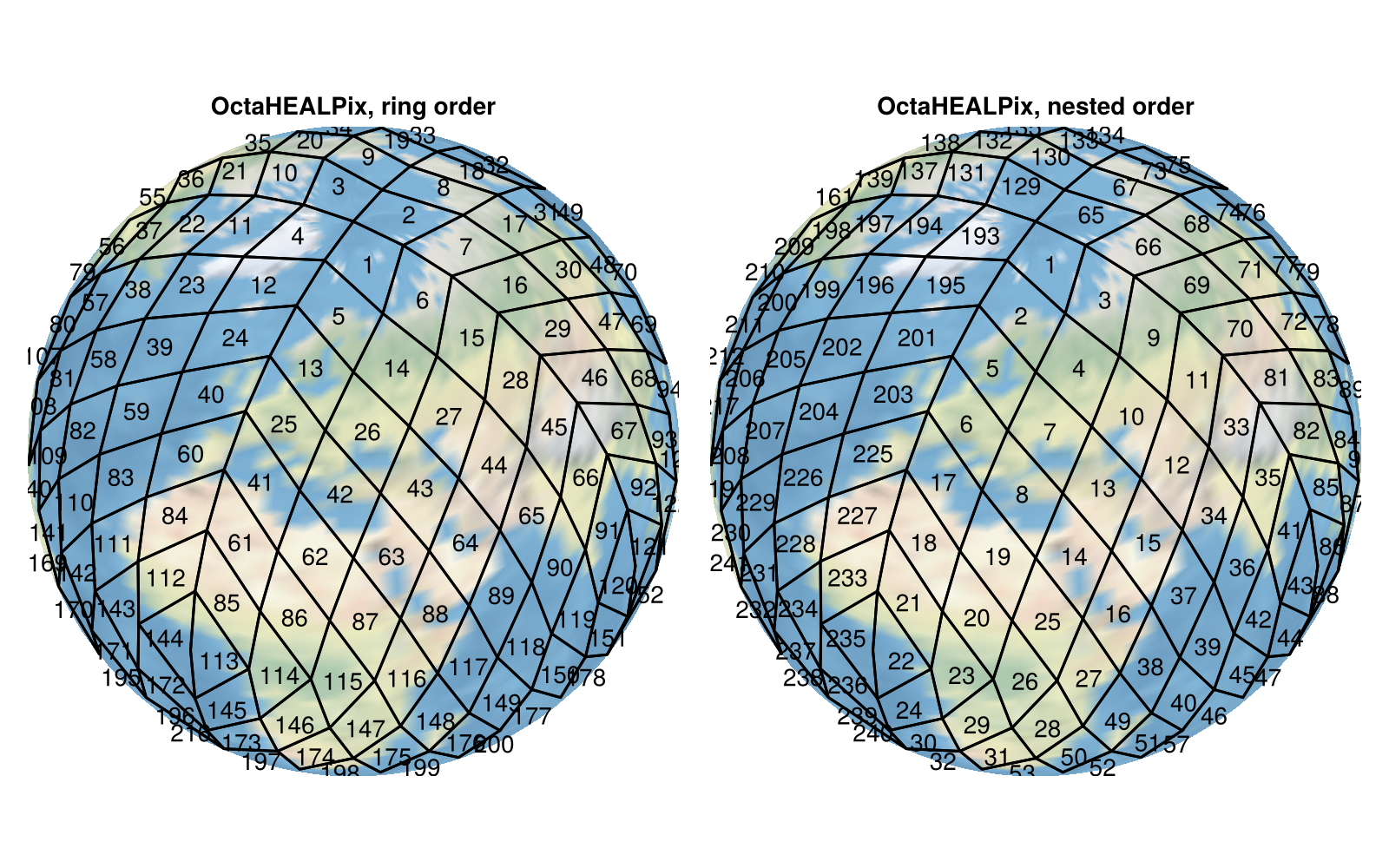
Copying unmasked grid points
Having a field and a mask on the same grid one can extract masked/unmasked elements (return as array) with field[mask] or field[.~mask], however, this operation allocates memory and it is not immediately possible to write the results of these operations allocation-free into existing arrays.
Hence, RingGrids provides unmasked_indices and copy_unmasked! that let you extract the unmasked subset of a ring-grid field into a (smaller) subset array, work on it, and scatter results back – allocation free on both CPU and GPU. Only a reusable indices vector has to be precomputed that maps the indices between the unmasked elements of the field to the contiguous elements in the array.
Convention: mask is a Bool field where true = masked (excluded), false = unmasked (included).
Start with a mask on a grid
grid = HEALPixGrid(2)
mask = rand(Bool, grid)                   # or use your own Bool field
12-element, 3-ring (XY) HEALPixField{Bool, 1} as Array on CPU
false
false
true
false
false
false
true
false
false
false
false
truePrecompute the indices to copy between field and array
indices = unmasked_indices(mask) # Vector of grid-point indices where mask == false9-element Vector{Int64}:
1
2
4
5
6
8
9
10
11indices lives on the same device as mask (CPU or GPU) and is sorted.
Now we can copy the unmasked elements of the field to the smaller plain array (gather):
field = rand(Float32, grid)12-element, 3-ring (XY) HEALPixField{Float32, 1} as Array on CPU
0.29134077f0
0.71357983f0
0.9685973f0
0.5526934f0
0.4205827f0
0.57019037f0
0.031863213f0
0.4946469f0
0.3306957f0
0.47395653f0
0.7265237f0
0.6626731f0The array must be of length n equal to the zero (=unmasked) elements in the mask
n = length(mask) - sum(mask)
array = zeros(Float32, n)
copy_unmasked!(array, field, indices)
array
9-element Vector{Float32}:
0.29134077
0.71357983
0.5526934
0.4205827
0.57019037
0.4946469
0.3306957
0.47395653
0.7265237Such that array is a subset of the elements in field. The unmasked values are identical
array == field[.~mask]trueSame works for 3D or higher dimensions, but the mask is always 2D
nlayers = 3
field3D = rand(Float32, grid, nlayers)
array3D = zeros(Float32, n, nlayers)
copy_unmasked!(array3D, field3D, indices)
9×3 Matrix{Float32}:
0.72642 0.0269923 0.229632
0.646031 0.62844 0.00706601
0.589521 0.00583369 0.458952
0.999985 0.831954 0.298125
0.036938 0.813107 0.380522
0.614593 0.841755 0.776289
0.658793 0.989636 0.632123
0.534078 0.676664 0.109309
0.779413 0.913202 0.955847And copy back, plain array → field (scatter):
other_field3D = zeros(Float32, grid, nlayers)
copy_unmasked!(other_field3D, array3D, indices)
field3D[.~mask, :] == other_field3D[.~mask, :]trueGrid points not referenced by indices (the masked ones) are left unchanged.
Function index
Core.Type Method
Create a new grid of type Grid with resolution parameter nlat_half. architecture is the device type (CPU/GPU). Precomputes the ring indices rings.
Core.Type Method
Zero generator function for the 4-point average AnvilLocator. Use update_locator! to update the grid indices used for interpolation and their weights. The number format NF is the format used for the calculations within the interpolation, the input data and/or output data formats may differ.
RingGrids.AbstractField Type
Abstract supertype for all fields, i.e. data on a grid. A field is an AbstractArray with a number format T, a number of dimensions N, an ArrayType (e.g. Vector, Matrix, Tensor) and a grid type Grid. Fields can be full or reduced, 2D, 3D, or 4D, depending on the grid and the number of dimensions. Fields are used to store data on the grid, e.g. temperature, pressure, or any other variable. Every Field has data the grid-free array of the data and grid which contains information about the grid the field is defined on.
RingGrids.AbstractField2D Type
Abstract supertype for all 2D fields, i.e. fields with the horizontal dimensions only. Note that this is a <:AbstractVector as the horizontal dimensions are unravelled into a vector for all grids to be conistent with the reduced grids that cannot be represented as a matrix.
RingGrids.AbstractField3D Type
Abstract supertype for all 3D fields, i.e. fields with horizontal and one vertical (or time etc) dimension.
sourceRingGrids.AbstractField4D Type
Abstract supertype for all 4D fields, i.e. fields with horizontal and (in most cases) a vertical and a time dimensions, though these additional dimensions are arbitrary.
sourceRingGrids.AbstractFieldWithTimeAndVertical Type
Abstract supertype for all fields with both time and vertical dimensions
sourceRingGrids.AbstractFieldWithVertical Type
Abstract supertype for all fields with a vertical dimension
sourceRingGrids.AbstractFullField Type
Abstract supertype for all fields on full grids, i.e. grids with a constant number of longitude points across latitude rings.
sourceRingGrids.AbstractFullGrid Type
Abstract supertype for all full grids, representing a horizontal grid with a constant number of longitude points across latitude rings. Different latitudes can be used, Gaussian latitudes, equi-angle latitudes (also called Clenshaw from Clenshaw-Curtis quadrature), or others.
sourceRingGrids.AbstractGrid Type
Abstract supertype for all grids in RingGrids.jl, representing a discretization (particularly a tessellation or tiling) of the sphere. A "grid" does not contain any data only its resolution is defined by nlat_half (number of latitude rings on one hemisphere including the equator). A grid does not contain the coordinates of the grid points, vertices, latitudes, longtiudes etc but they can be recomputed from the grid object (or its type and resolution) at any time.
A grid is regarded as 2D but a field (data on a grid) can have N additional dimensions, e.g. for vertical levels or time. In that sense, a grid does not have a number format / eltype. This is a property of a Field which can be different for every field even when using the same grid. Points on the grid (cell centres) are unravalled into a vector ordered 0 to 360˚E, starting at the north pole, then going ring by ring to the south pole. This way both full (those representable as a matrix) and reduced grids (not representable as a matrix, with fewer longitude points towards the poles) can be represented.
A grid has a parameter Architecture (the type of the field architecture) that can be used to store information about the architecture the grid is on, e.g. CPU or GPU.
Furthermore all grids have a rings to allow ring-by-ring indexing. Other precomputed indices can be added for specific grids.
RingGrids.AbstractInterpolator Type
abstract type AbstractInterpolator endSupertype for Interpolators. Every Interpolator <: AbstractInterpolator is expected to have two fields,
geometry, which describes the grid G to interpolate from
locator, which locates the indices on G and their weights to interpolate onto a new grid.
NF is the number format used to calculate the interpolation, which can be different from the input data and/or the interpolated data on the new grid.
sourceRingGrids.AbstractLocator Type
Supertype of every Locator, which locates the indices on a grid to be used to perform an interpolation. E.g. AnvilLocator uses a 4-point stencil for every new coordinate to interpolate onto. Higher order stencils can be implemented by defining OtherLocator <: AbstractLocactor.
sourceRingGrids.AbstractReducedField Type
Abstract supertype for all fields on reduced grids, i.e. grids with a reduced number of longitude points towards the poles.
sourceRingGrids.AbstractReducedGrid Type
Abstract supertype for all reduced grids, representing arrays of ring grids that have a reduced number of longitude points towards the poles, i.e. they are not "full", see AbstractFullGrid. Data on these grids (a Field) cannot be represented as matrix and has to be unravelled into a vector, ordered 0 to 360˚E then north to south, ring by ring. Examples for reduced grids are the octahedral Gaussian or Clenshaw grids, or the HEALPix grid.
RingGrids.AbstractSphericalDistance Type
abstract type AbstractSphericalDistance endSuper type of formulas to calculate the spherical distance or great-circle distance. To define a NewFormula, define struct NewFormula <: AbstractSphericalDistance end and the actual calculation as a functor
function NewFormula(lonlat1::Tuple, lonlat2::Tuple; radius=DEFAULT_RADIUS, kwargs...)assuming inputs in degrees and returning the distance in meters (or radians for radius=1). Then use the general interface spherical_distance(NewFormula, args...; kwargs...)
RingGrids.AnvilInterpolator Type
Interpolator type for anvil_average.
NF is the number format used to calculate the interpolation, which can be different from the input data and/or the interpolated data on the new grid.
sourceRingGrids.AnvilLocator Type
Contains arrays that locates grid points of a given field to be uses in an interpolation and their weights. This Locator is a 4-point average in an anvil-shaped grid-point arrangement between two latitude rings.
sourceRingGrids.ColumnField Type
ColumnField is a version of Field with data stored in a column-major format. It is used e.g. to represent data on a vertical column of a grid in column-based parametrizations.
data::AbstractArraygrid::AbstractGriddims::Any
A ColumnField can be easily created from a Field by transposing it:
field = Field(grid, k...)
column_field = transpose(field)RingGrids.Field Type
Field contains data on a grid. There is only one Field type which can be used for all grids. data is the data array, the first dimension is always the horizontal dimension (unravelled into a vector for compatibility across full and reduced grids), the other dimensions can be used for the vertical and/or time or other dimensions. The grid can be shared across multiple fields, e.g. a 2D and a 3D field can share the same grid which just defines the discretization and the architecture (CPU/GPU) the grid is on.
data::AbstractArraygrid::AbstractGriddims::SpeedyWeatherInternals.ArrayDimensions.AbstractArrayDimensions
RingGrids.FullClenshawGrid Type
A FullClenshawGrid is a discretization of the sphere, a full grid, subtyping AbstractFullGrid, using equidistant latitudes for each ring (a regular lon-lat grid). These require the Clenshaw-Curtis quadrature in the spectral transform, hence the name. One ring is on the equator, total number of rings is odd, no rings on the north or south pole.
The first dimension of data on this grid (a Field) represents the horizontal dimension, in ring order (0 to 360˚E, then north to south), other dimensions can be used for the vertical and/or time or other dimensions. Note that a Grid does not contain any data, it only describes the discretization of the space, see Field for a data on a Grid. But a "grid" only defines the two horizontal dimensions, two fields, one 2D and one 3D, possibly different ArrayTypes or element types, can share the same grid which just defines the discretization and the architecture (CPU/GPU) the grid is on.
The resolution parameter of the horizontal grid is nlat_half (number of latitude rings on one hemisphere, Equator included) and the ring indices are precomputed in rings.
nlat_half::Anyarchitecture::Anyrings::Anywhichring::Any
RingGrids.FullGaussianGrid Type
A FullGaussianGrid is a discretization of the sphere that uses Gaussian latitudes for each latitude ring. As a "full" grid it has the same number of longitude points on every latitude ring, i.e. it is representable as a matrix, with denser grid points towards the poles. The Gaussian latitudes enable to use the Gaussian quadrature for the spectral transform, hence the name. No ring is on the equator, total number of rings is even and symmetric around the Equator, no rings on the north or south pole.
The first dimension of data on this grid (a Field) represents the horizontal dimension, in ring order (0 to 360˚E, then north to south), other dimensions can be used for the vertical and/or time or other dimensions. Note that a Grid does not contain any data, it only describes the discretization of the space, see Field for a data on a Grid. But a "grid" only defines the two horizontal dimensions, two fields, one 2D and one 3D, possibly different ArrayTypes or element types, can share the same grid which just defines the discretization and the architecture (CPU/GPU) the grid is on.
The resolution parameter of the horizontal grid is nlat_half (number of latitude rings on one hemisphere, Equator included) and the ring indices are precomputed in rings.
nlat_half::Anyarchitecture::Anyrings::Anywhichring::Any
RingGrids.FullHEALPixGrid Type
A FullHEALPixGrid is like a HEALPixGrid but with every latitude ring having the same number of longitude points (a full grid). This grid is mostly defined for output to minimize the interpolation needed from a HEALPixGrid to a full grid. A FullHEALPixGrid has none of the equal-area properties of the HEALPixGrid. It only shares the latitudes with the HEALPixGrid but uses the longitudes from the FullGaussianGrid without offset, i.e. the first longitude point on every ring is at 0˚E.
nlat_half::Anyarchitecture::Anyrings::Anywhichring::Any
RingGrids.FullOctaHEALPixGrid Type
A FullOctaHEALPixGrid is like a OctaHEALPixGrid but with every latitude ring having the same number of longitude points (a full grid). This grid is mostly defined for output to minimize the interpolation needed from an OctaHEALPixGrid to a full grid required for output. A FullOctaHEALPixGrid has none of the equal-area properties of the OctaHEALPixGrid. It only shares the latitudes with the OctaHEALPixGrid but uses the longitudes from the FullGaussianGrid without offset, i.e. the first longitude point on every ring is at 0˚E.
nlat_half::Anyarchitecture::Anyrings::Anywhichring::Any
RingGrids.GridGeometry Type
Contains general precomputed arrays describing the grid.
grid::Anynlat_half::Anynlat::Anynpoints::Anylonds::Anylatd::Anynlons::Anylon_offsets::Anyrings::Any
RingGrids.GridGeometry Method
GridGeometry(
    grid::AbstractGrid;
    NF
) -> GridGeometry{<:AbstractGrid{Architecture}, Vector{Float32}, Vector{Int64}} where Architecture
Precomputed arrays describing the geometry of the Grid with resolution nlat_half. Contains longitudes, latitudes of grid points, their ring index j and their unravelled indices ij.
RingGrids.HEALPixGrid Type
A HEALPixGrid is a equal-area discretization of the sphere. A HEALPix grid has 12 faces, each nsidexnside grid points, each covering the same area of the sphere. They start with 4 longitude points on the northern-most ring, increase by 4 points per ring in the "polar cap" (the top half of the 4 northern-most faces) but have a constant number of longitude points in the equatorial belt. The southern hemisphere is symmetric to the northern, mirrored around the Equator. HEALPix grids have a ring on the Equator. For more details see Górski et al. 2005, DOI:10.1086/427976.
rings are the precomputed ring indices, for nlat_half = 4 it is rings = [1:4, 5:12, 13:20, 21:28, 29:36, 37:44, 45:48]. So the first ring has indices 1:4 in the unravelled first dimension, etc. For efficient looping see eachring and eachgrid. whichring is a precomputed vector of ring indices for each grid point ij, i.e. whichring[ij] gives the ring index j of grid point ij. Fields are
nlat_half::Anyarchitecture::Anyrings::Anywhichring::Any
RingGrids.Haversine Method
Haversine(lonlat1::Tuple, lonlat2::Tuple; radius) -> AnyHaversine formula calculating the great-circle or spherical distance (in meters) on the sphere between two tuples of longitude-latitude points in degrees ˚E, ˚N. Use keyword argument radius to change the radius of the sphere (default 6371e3 meters, Earth's radius), use radius=1 to return the central angle in radians or radius=360/2π to return degrees.
RingGrids.OctaHEALPixGrid Type
An OctaHEALPixGrid is an equal-area discretization of the sphere. It has 4 faces, each nlat_half x nlat_half in size, covering 90˚ in longitude, pole to pole. As part of the HEALPix family of grids, the grid points are equal area. They start with 4 longitude points on the northern-most ring, increase by 4 points per ring towards the Equator with one ring on the Equator before reducing the number of points again towards the south pole by 4 per ring. There is no equatorial belt for OctaHEALPix grids. The southern hemisphere is symmetric to the northern, mirrored around the Equator. OctaHEALPix grids have a ring on the Equator. For more details see Górski et al. 2005, DOI:10.1086/427976, the OctaHEALPix grid belongs to the family of HEALPix grids with Nθ = 1, Nφ = 4 but is not explicitly mentioned therein.
rings are the precomputed ring indices, for nlat_half = 3 (in contrast to HEALPix this can be odd) it is rings = [1:4, 5:12, 13:24, 25:32, 33:36]. For efficient looping see eachring and eachgrid. whichring is a precomputed vector of ring indices for each grid point ij, i.e. whichring[ij] gives the ring index j of grid point ij. Fields are
nlat_half::Anyarchitecture::Anyrings::Anywhichring::Any
RingGrids.OctahedralClenshawGrid Type
An OctahedralClenshawGrid is a discretization of the sphere that uses equidistant latitudes for each latitude ring. The spherical harmonic transform on this grid uses the Clenshaw-Curtis quadrature, hence the name. As a reduced grid it has a different number of longitude points on every latitude ring. These grids are called octahedral because after starting with 20 points on the first ring around the north pole they increase the number of longitude points for each ring by 4, such that they can be conceptually thought of as lying on the 4 faces of an octahedron on each hemisphere. Hence, these grids have 20, 24, 28, ... longitude points for ring 1, 2, 3, ... There is a ring on the Equator with 16 + 4nlat_half longitude points before reducing the number of longitude points per ring by 4 towards the southern-most ring j = nlat. The first point on every ring is at longitude 0˚E, i.e. no offset is applied to the longitude values (in contrast to HEALPix grids).
The first dimension of data on this grid (a Field) represents the horizontal dimension, in ring order (0 to 360˚E, then north to south), other dimensions can be used for the vertical and/or time or other dimensions. Note that a Grid does not contain any data, it only describes the discretization of the space, see Field for a data on a Grid. But a "grid" only defines the two horizontal dimensions, two fields, one 2D and one 3D, possibly different ArrayTypes or element types, can share the same grid which just defines the discretization and the architecture (CPU/GPU) the grid is on.
The resolution parameter of the horizontal grid is nlat_half (number of latitude rings on one hemisphere, Equator included) rings are the precomputed ring indices, the the example above rings = [1:20, 21:44, 45:72, ...]. whichring is a precomputed vector of ring indices for each grid point ij, i.e. whichring[ij] gives the ring index j of grid point ij. For efficient looping see eachring and eachgrid. Fields are
nlat_half::Anyarchitecture::Anyrings::Anywhichring::Any
RingGrids.OctahedralGaussianGrid Type
An OctahedralGaussianGrid is a discretization of the sphere that uses Gaussian latitudes for each latitude ring. As a reduced grid it has a different number of longitude points on every latitude ring. These grids are called octahedral because after starting with 20 points on the first ring around the north pole they increase the number of longitude points for each ring by 4, such that they can be conceptually thought of as lying on the 4 faces of an octahedron on each hemisphere. Hence, these grids have 20, 24, 28, ... longitude points for ring 1, 2, 3, ... There is no ring on the Equator and the two rings around it have 16 + 4nlat_half longitude points before reducing the number of longitude points per ring by 4 towards the southern-most ring j = nlat. The first point on every ring is at longitude 0˚E, i.e. no offset is applied to the longitude values (in contrast to HEALPix grids).
The first dimension of data on this grid (a Field) represents the horizontal dimension, in ring order (0 to 360˚E, then north to south), other dimensions can be used for the vertical and/or time or other dimensions. Note that a Grid does not contain any data, it only describes the discretization of the space, see Field for a data on a Grid. But a "grid" only defines the two horizontal dimensions, two fields, one 2D and one 3D, possibly different ArrayTypes or element types, can share the same grid which just defines the discretization and the architecture (CPU/GPU) the grid is on.
The resolution parameter of the horizontal grid is nlat_half (number of latitude rings on one hemisphere, Equator included) rings are the precomputed ring indices, the the example above rings = [1:20, 21:44, 45:72, ...]. whichring is a precomputed vector of ring indices for each grid point ij, i.e. whichring[ij] gives the ring index j of grid point ij. For efficient looping see eachring and eachgrid. Fields are
nlat_half::Anyarchitecture::Anyrings::Anywhichring::Any
RingGrids.OctaminimalGaussianGrid Type
An OctaminimalGaussianGrid is a discretization of the sphere that uses Gaussian latitudes for each latitude ring. It is very similar to the OctahedralGaussianGrid, with a few differences: 2. It starts with 4 longitude points around the poles, so 4, 8, 12, 16, ... on ring 1, 2, 3, 4, ... reducing the number
of total number of grid points over the OctahedralGaussianGrid, hence the name "octaminimal" (octahedral minimal). 2. The first longitude points on every ring have an offset, such that the cell face between the first and last longitude point on every ring is at 0˚E (like the HEALPix grid)
Fields are
nlat_half::Anyarchitecture::Anyrings::Anywhichring::Any
Base._reverse! Method
_reverse!(field::AbstractField, sym::Symbol) -> AnyReverse field in-place along dimension sym, called via reverse!(field, dims=:lat). :lat (or :latitude) mirrors the field about the equator, :lon (or :longitude) reverses the direction of every ring.
Base._reverse! Method
_reverse!(
    field::AbstractField,
    _::Val{:lat}
) -> AbstractField
Mirror field about the equator in-place by swapping every northern ring with its southern counterpart, as called via reverse!(field, dims=:lat).
Base._reverse! Method
_reverse!(
    field::AbstractField,
    _::Val{:lon}
) -> AbstractField
Reverse field in longitude in-place (mirror at the 0˚ meridian), as called via reverse!(field, dims=:lon). On rings with a longitudinal offset (first point dlon/2 east of 0˚, see hasoffset) all points within the ring are reversed; on rings whose first point lies on 0˚ that point stays and only the remaining points are reversed. Either way the ring is mirrored exactly at 0˚, consistent with the spectral reverse!(::LowerTriangularArray, dims=:lon).
LinearAlgebra.rotate! Method
rotate!(field::AbstractField, degree::Integer) -> AnyRotate field eastward in longitude by degree in-place, a multiple of 90˚ (negative degrees rotate westward). Every ring is circularly shifted by the corresponding number of quarter rings.
RingGrids._scale_lat! Method
_scale_lat!(
    field::AbstractField,
    v::AbstractVector
) -> AbstractField
Generic latitude scaling applied to field in-place with latitude-like vector v.
RingGrids.anvil_average Method
anvil_average(a, b, c, d, Δab, Δcd, Δy) -> AnyThe bilinear average of a, b, c, d which are values at grid points in an anvil-shaped configuration at location x, which is denoted by Δab, Δcd, Δy, the fraction of distances between a-b, c-d, and ab-cd, respectively. Note that a, c and b, d do not necessarily share the same longitude/x-coordinate. See schematic:
            0..............1    # fraction of distance Δab between a, b
            |<  Δab   >|

    0^      a -------- o - b    # anvil-shaped average of a, b, c, d at location x
    .Δy                |
    .                  |
    .v                 x
    .                  |
    1         c ------ o ---- d

              |<  Δcd >|
              0...............1 # fraction of distance Δcd between c, d
^ fraction of distance Δy between a-b and c-d.
sourceRingGrids.average_on_poles Method
average_on_poles(
    A::AbstractArray{NF<:AbstractFloat, 1},
    rings
) -> Tuple{Any, Any}
Computes the average at the North and South pole from a given grid A and it's precomputed ring indices rings. The North pole average is an equally weighted average of all grid points on the northern-most ring. Similar for the South pole.
RingGrids.average_on_poles Method
average_on_poles(
    A::AbstractArray{NF<:Integer, 1},
    rings
) -> Tuple{Any, Any}
Method for A::Abstract{T<:Integer} which rounds the averaged values to return the same number format NF.
RingGrids.clenshaw_curtis_weights Method
clenshaw_curtis_weights(nlat_half::Integer) -> AnyThe Clenshaw-Curtis weights for a Clenshaw grid (full or octahedral) of size nlat_half. Clenshaw-Curtis weights are of length nlat, i.e. a vector for every latitude ring, pole to pole. sum(clenshaw_curtis_weights(nlat_half)) is always 2 as
Integration (and therefore the spectral transform) is exact (only rounding errors) when using Clenshaw grids provided that nlat >= 2(T + 1), meaning that a grid resolution of at least 128x64 (nlon x nlat) is sufficient for an exact transform with a T=31 spectral truncation.
RingGrids.copy_unmasked! Method
copy_unmasked!(
    dst::AbstractArray,
    src::AbstractField,
    indices
) -> AbstractArray
Copy a subset of grid points from the ring-grid Field src into the plain array dst, where indices maps each row of dst to the corresponding flat grid-point index in src. indices is typically produced by unmasked_indices.
The first dimension of dst and indices must match (the number of unmasked points); remaining dimensions are treated as vertical layers and are copied verbatim.
RingGrids.copy_unmasked! Method
copy_unmasked!(
    dst::AbstractField,
    src::AbstractArray,
    indices
) -> AbstractField
Reverse of the field→array method: scatter the rows of the plain array src back into the ring-grid Field dst at the positions given by indices. Grid points not referenced by indices are left unchanged. indices is typically produced by unmasked_indices.
RingGrids.deinterleave Method
deinterleave(ui::Integer) -> AnyDeinterleave an integer's bits, e.g.
00000000 00000000 00000000 00010101becomes
00000000 00000000 00000000 00000111.RingGrids.each_index_in_ring! Method
each_index_in_ring!(
    rings,
    Grid::Type{<:OctahedralGaussianGrid},
    nlat_half::Integer
)
precompute a Vector{UnitRange{Int}} to index grid points on every ringj(elements of the vector) ofGridat resolutionnlat_half. Seeeachringandeachgrid` for efficient looping over grid points.
RingGrids.each_index_in_ring! Method
each_index_in_ring!(
    rings,
    Grid::Type{<:OctaminimalGaussianGrid},
    nlat_half::Integer
)
precompute a Vector{UnitRange{Int}} to index grid points on every ringj(elements of the vector) ofGridat resolutionnlat_half. Seeeachringandeachgrid` for efficient looping over grid points.
RingGrids.each_index_in_ring Method
each_index_in_ring(grid::AbstractGrid, j::Integer) -> AnyUnitRange to access data on grid grid on ring j.
RingGrids.each_index_in_ring Method
each_index_in_ring(
    Grid::Type{<:AbstractFullGrid},
    j::Integer,
    nlat_half::Integer
) -> Any
UnitRange for every grid point of full grid Grid of resolution nlat_half on ring j (j=1 is closest ring around north pole, j=nlat around south pole).
RingGrids.eachgridpoint Method
eachgridpoint(
    field1::AbstractField,
    fields::AbstractField...;
    horizontal_only,
    kwargs...
) -> Any
Iterator over all 2D grid points of a field (or fields), i.e. the horizontal dimension only. Intended use is like
for ij in eachgridpoint(field)
    field[ij]
for a 2D field. For a 3D+ field, the iterator will only index and loop over the horizontal grid points. If horizontal_only is set to true (default), the function will only check whether the horizontal dimensions match.
RingGrids.eachgridpoint Method
eachgridpoint(
    grid1::AbstractGrid,
    grids::AbstractGrid...
) -> Any
Like eachgridpoint(::AbstractGrid) but checks grids match.
RingGrids.eachgridpoint Method
eachgridpoint(grid::AbstractGrid) -> AnyUnitRange to access each horizontal grid point on grid grid. For a NxM (N horizontal grid points, M vertical layers) OneTo(N) is returned.
RingGrids.eachlayer Method
eachlayer(
    field1::AbstractField,
    fields::AbstractField...;
    vertical_only,
    kwargs...
) -> Any
CartesianIndices for the 2nd to last dimension of a field (or fields), e.g. the vertical layer (and possibly a time dimension, etc). E.g. for a Nx2x3 field, with N horizontal grid points k iterates over (1, 1) to (2, 3), meaning both the 2nd and 3rd dimension. To be used like
for k in eachlayer(field)
    for (j, ring) in enumerate(eachring(field))
        for ij in ring
            field[ij, k]
With vertical_only=true (default) only checks whether the non-horizontal dimensions of the fields match. E.g. one can loop over two fields of each n layers on different grids.
RingGrids.eachring Method
eachring(
    field1::AbstractField,
    fields::AbstractField...;
    horizontal_only,
    kwargs...
) -> Any
Return an iterator over the rings of a field. These are precomputed ranges like [1:20, 21:44, ...] stored in field.grid.rings. Every element are the unravellend indices ij of all 2D grid points that lie on that ring. Intended use is like
for (j, ring) in enumerate(eachring(field))
    for ij in ring
        field[ij, k]
with j being the ring index. j=1 around the north pole, j=nlat_half around the Equator or just north of it (for even nlat_half). Several fields can be passed on to check for matching grids, e.g. for a 2D and a 3D field. If horizontal_only is set to true, the function will only check the horizontal dimension.
RingGrids.eachring Method
eachring(grid1::AbstractGrid, grids::AbstractGrid...) -> AnySame as eachring(grid) but performs a bounds check to assess that all grids according to grids_match (non-parametric grid type, nlat_half and length).
RingGrids.eachring Method
eachring(grid::AbstractGrid) -> AnyVector{UnitRange} rings to loop over every ring of grid and then each grid point per ring. To be used like
rings = eachring(grid)
for ring in rings
    for ij in ring
        field[ij]
Accesses precomputed grid.rings.
RingGrids.eachring Method
eachring(
    Grid::Type{<:AbstractGrid},
    nlat_half::Integer
) -> Any
Computes the ring indices i0:i1 for start and end of every longitudinal point on a given ring j of Grid at resolution nlat_half. Used to loop over rings of a grid. These indices are also precomputed in every grid.rings.
RingGrids.eachring_on_architecture Method
eachring_on_architecture(
    arch,
    grid::AbstractGrid
) -> Tuple{Any, Any}
First index and length of every ring in grid as two vectors on architecture arch, for use inside kernels where the CPU-only grid.rings is unavailable.
RingGrids.equal_area_weights Method
equal_area_weights(
    Grid::Type{<:AbstractGrid},
    nlat_half::Integer
) -> Any
The equal-area weights used for the HEALPix grids (original or OctaHEALPix) of size nlat_half. The weights are of length nlat, i.e. a vector for every latitude ring, pole to pole. sum(equal_area_weights(nlat_half)) is always 2 as
RingGrids.extrema_in Method
extrema_in(v::AbstractVector, a::Real, b::Real) -> AnyFor every element vᵢ in v does a<=vi<=b hold?
sourceRingGrids.fields_match Method
fields_match(
    A::AbstractField,
    B::AbstractField;
    horizontal_only,
    vertical_only
) -> Any
True if both A and B are of the same nonparametric grid type (e.g. OctahedralGaussianArray, regardless type parameter T or underyling array type ArrayType) and of same resolution (nlat_half) and total grid points (length). Sizes of (4,) and (4,1) would match for example, but (8,1) and (4,2) would not (nlat_half not identical).
RingGrids.gaussian_weights Method
gaussian_weights(nlat_half::Integer) -> AnyThe Gaussian weights for a Gaussian grid (full or octahedral) of size nlat_half. Gaussian weights are of length nlat, i.e. a vector for every latitude ring, pole to pole. sum(gaussian_weights(nlat_half)) is always 2 as
Integration (and therefore the spectral transform) is exact (only rounding errors) when using Gaussian grids provided that nlat >= 3(T + 1)/2, meaning that a grid resolution of at least 96x48 (nlon x nlat) is sufficient for an exact transform with a T=31 spectral truncation.
RingGrids.get_asset Method
get_asset(
    path::String;
    from_assets,
    name,
    ArrayType,
    FileFormat,
    assets_url,
    version,
    fill_value,
    output_grid
)
Downloads a file under path from an assets repository (if from_assets=true, otherwise loads locally), adds it to Artifacts.toml in the package directory, and returns the loaded data. Use version = "branch" (a String) to retrieve data from a branch, e.g. version = "main" for the latest on the main branch. name is used to find a variable inside the file, ArrayType to determine how to wrap the loaded data (in most cases into a Field subtype, determining the grid). FileFormat determines how to read the file; load NCDatasets.jl to enable reading NetCDF files. assets_url can be set to a custom URL for alternative asset repositories (e.g. for Terrarium). version is the version tag (a VersionNumber) or branch name (a String) to download from. fill_value is the value used to replace missing data (identified by the file's _FillValue attribute) in the loaded array; defaults to NaN. output_grid is the grid to interpolate the loaded data to; defaults to nothing (no interpolation). ArrayType must be a AbstractFullField type for interpolation to work.
RingGrids.get_colat Method
get_colat(grid::AbstractGrid) -> AnyColatitudes (radians) for each ring in grid, north to south.
RingGrids.get_gridcell_polygons Method
get_gridcell_polygons(
    Grid::Type{<:AbstractGrid},
    nlat_half::Integer;
    add_nan
) -> Matrix{Tuple{Float64, Float64}}
Return a 5xN matrix polygons (or grid cells) of NTuple{2, Float64} where the first 4 rows are the vertices (E, S, W, N) of every grid points ij in 1:N, row 5 is duplicated north vertex to close the grid cell. Use keyword argument add_nan=true (default false) to add a 6th row with (NaN, NaN) to separate grid cells when drawing them as a continuous line with vec(polygons).
RingGrids.get_lat Method
get_lat(grid::AbstractGrid) -> AnyLatitude (radians) for each ring in grid, north to south.
RingGrids.get_latd Method
get_latd(grid::AbstractGrid) -> AnyLatitude (degrees) for each ring in grid, north to south.
RingGrids.get_latd Method
get_latd(_::Type{<:HEALPixGrid}, nlat_half::Integer) -> AnyLatitudes [90˚N to -90˚N] for the HEALPixGrid with resolution parameter nlat_half.
RingGrids.get_lon Method
get_lon(grid::AbstractGrid) -> AnyLongitude (radians). Full grids only.
sourceRingGrids.get_loncolats Method
get_loncolats(grid::AbstractGrid) -> Tuple{Any, Any}Longitudes (radians, 0-2π), colatitudes (degrees, 0 to π) for every (horizontal) grid point in grid in ring order (0-360˚E then north to south).
RingGrids.get_lond Method
get_lond(grid::AbstractGrid) -> AnyLongitude (degrees). Full grids only.
sourceRingGrids.get_lond_per_ring Method
get_lond_per_ring(
    Grid::Type{<:HEALPixGrid},
    nlat_half::Integer,
    j::Integer
) -> Any
Longitudes [0˚E to 360˚E] for the HEALPixGrid with resolution parameter nlat_half on ring j (north to south).
RingGrids.get_londlatds Method
get_londlatds(grid::AbstractGrid) -> Tuple{Any, Any}Longitudes (degrees, 0-360˚E), latitudes (degrees, 90˚N to -90˚N) for every (horizontal) grid point in grid in ring order (0-360˚E then north to south).
RingGrids.get_londlatds Method
get_londlatds(
    Grid::Type{<:AbstractReducedGrid},
    nlat_half::Integer
) -> Tuple{Any, Any}
Return vectors of londs, latds, of longitudes (degrees, 0-360˚E) and latitudes (degrees, -90˚ to 90˚N) for reduced grids for all grid points in order of the running index ij.
RingGrids.get_lonlats Method
get_lonlats(grid::AbstractGrid) -> Tuple{Any, Any}Longitudes (radians, 0-2π), latitudes (degrees, π/2 to -π/2) for every (horizontal) grid point in grid in ring order (0-360˚E then north to south).
RingGrids.get_nlat Method
get_nlat(grid::AbstractGrid) -> AnyGet number of latitude rings, pole to pole.
sourceRingGrids.get_nlat_half Method
get_nlat_half(grid::AbstractGrid) -> AnyResolution parameters nlat_half of a grid. Number of latitude rings on one hemisphere, Equator included.
RingGrids.get_nlon_per_ring Method
get_nlon_per_ring(grid::AbstractGrid, j::Integer) -> AnyNumber of longitude points per latitude ring j.
RingGrids.get_nlon_per_ring Method
get_nlon_per_ring(
    Grid::Type{<:HEALPixGrid},
    nlat_half::Integer,
    j::Integer
) -> Any
Number of longitude points for ring j on Grid of resolution nlat_half.
RingGrids.get_nlons Method
get_nlons(
    Grid::Type{<:AbstractGrid},
    nlat_half::Integer;
    both_hemispheres
) -> Any
Returns a vector nlons for the number of longitude points per latitude ring, north to south. Provide grid Grid and its resolution parameter nlat_half. For keyword argument both_hemispheres=false only the northern hemisphere (incl Equator) is returned.
RingGrids.get_npoints Method
get_npoints(grid::AbstractGrid, args...) -> AnyTotal number of grid points in all dimensions of grid. Equivalent to length of the underlying data array.
RingGrids.get_vertices Method
get_vertices(
    Grid::Type{<:AbstractFullGrid},
    nlat_half::Integer
) -> NTuple{4, Any}
Vertices for full grids, other definition than for reduced grids to prevent a diamond shape of the cells. Use default rectangular instead. Effectively rotating the vertices clockwise by 45˚, making east south-east etc.
sourceRingGrids.get_vertices Method
get_vertices(
    Grid::Type{<:AbstractGrid},
    nlat_half::Integer
) -> NTuple{4, Any}
Vertices are defined for every grid point on a ring grid through 4 points: east, south, west, north.
east: longitude mid-point with the next grid point east
south: longitude mid-point between the two closest grid points on one ring to the south
west: longitude mid-point with the next grid point west
north: longitude mid-point between the two closest grid points on one ring to the north
Example
   o ----- n ------ o

o --- w --- c --- e --- o

     o ----- s ------ o
with cell center c (the grid point), e, s, w, n the vertices and o the surrounding grid points. Returns 2 x npoints arrays for east, south, west, north each containing the longitude and latitude of the vertices.
sourceRingGrids.grid_cell_average! Method
grid_cell_average!(
    output::Field,
    input::AbstractField{T, N, ArrayType, Grid} where {T, N, ArrayType, Grid<:AbstractFullGrid}
) -> Field
Averages all grid points in input that are within one grid cell of output with coslat-weighting. The output grid cell boundaries are assumed to be rectangles spanning half way to adjacent longitude and latitude points.
RingGrids.grid_cell_average Method
grid_cell_average(
    Grid::Type{<:AbstractGrid},
    nlat_half::Integer,
    input::AbstractFullGrid
)
Averages all grid points in input that are within one grid cell of output with coslat-weighting. The output grid cell boundaries are assumed to be rectangles spanning half way to adjacent longitude and latitude points.
RingGrids.grids_match Method
grids_match(A::AbstractGrid, B::AbstractGrid) -> AnyTrue if both A and B are of the same nonparametric grid type (e.g. OctahedralGaussianArray, regardless type parameter T or underyling array type ArrayType) and of same resolution (nlat_half) and total grid points (length). Sizes of (4,) and (4,1) would match for example, but (8,1) and (4,2) would not (nlat_half not identical).
RingGrids.grids_match Method
grids_match(A::AbstractGrid, Bs::AbstractGrid...) -> AnyTrue if all grids A, B, C, ... provided as arguments match according to grids_match wrt to A (and therefore all).
RingGrids.grids_match Method
grids_match(
    A::Type{<:AbstractGrid},
    B::Type{<:AbstractGrid}
) -> Any
True if both A and B are of the same nonparametric grid type.
RingGrids.hasoffset Method
hasoffset(grid::AbstractGrid) -> AnyTrue if the first longitude point on every ring of the grid is offset half a longitudinal grid spacing east of the 0˚ meridian, false if the first point lies on 0˚ exactly. Defined per grid type; grids where only some rings have an offset (HEALPixGrid) only define the per-ring hasoffset(Grid, nlat_half, j).
RingGrids.hasoffset Method
hasoffset(
    Grid::Type{<:AbstractGrid},
    nlat_half::Integer,
    j::Integer
) -> Any
Like hasoffset(grid) but for ring j, for grids like HEALPixGrid where only some rings have a longitudinal offset.
RingGrids.interleave_with_zeros Method
interleave_with_zeros(ui::Integer) -> AnyInterleave an integer's bits with zeros, e.g.
00000000 00000000 00000000 00000111becomes
00000000 00000000 00000000 00010101The highest half of the bits are zeros will be discarded.
sourceRingGrids.matrix_size Method
matrix_size(grid::AbstractGrid) -> Tuple{Any, Any}Size of the matrix of the horizontal grid if representable as such (not all grids).
sourceRingGrids.nest2rcq Method
nest2rcq(ij, nside) -> Tuple{Any, Any, Any}Convert nested index ij to matrix indices row, column (r, c) and quadrant q. All 1-based. r=1, c=1, is at the north pole, r increases south-eastwards, c increases south-westwards. Quadrants are numbered 1 to 4 starting at the prime meridian and increasing eastwards.
sourceRingGrids.nest2ring Method
nest2ring(ij::Integer, grid::OctaHEALPixGrid) -> AnyConvert nested index ij to ring index ij of grid. All 1-based.
sourceRingGrids.nlat_odd Method
nlat_odd(grid::AbstractGrid) -> AnyTrue for a grid that has an odd number of latitude rings nlat (both hemispheres).
RingGrids.nside_healpix Method
nside_healpix(nlat_half::Integer) -> AnyThe original Nside resolution parameter of the HEALPix grids. The number of grid points on one side of each (square) face. While we use nlat_half across all ring grids, this function translates this to Nside. Even nlat_half only.
RingGrids.offset_maybe_vector Method
offset_maybe_vector(arch, grid::AbstractGrid) -> AnyThe longitudinal offset of grid as passed to kernels: hasoffset(grid) as a scalar Bool for grids where it is identical on every ring, but a Bool vector (one per ring, on architecture arch) for grids like HEALPixGrid where it is ring-dependent.
RingGrids.rcq2nest Method
rcq2nest(r, c, q, nside::Integer) -> AnyConvert matrix indices row, column (r, c) and quadrant q to nested index ij. All 1-based. r=1, c=1, is at the north pole, r increases south-eastwards, c increases south-westwards. Quadrants are numbered 1 to 4 starting at the prime meridian and increasing eastwards.
sourceRingGrids.rcq2ring Method
rcq2ring(r, c, q, grid::OctaHEALPixGrid) -> AnyConvert matrix indices row, column (r, c) and quadrant q to ring index ij. All 1-based. r=1, c=1, is at the north pole, r increases south-eastwards, c increases south-westwards. Quadrants are numbered 1 to 4 starting at the prime meridian and increasing eastwards.
sourceRingGrids.ring2nest Method
ring2nest(ij::Integer, grid::OctaHEALPixGrid) -> AnyConvert ring index ij to nested index ij of grid. All 1-based.
sourceRingGrids.ring2rcq Method
ring2rcq(
    ij::Integer,
    grid::OctaHEALPixGrid
) -> Tuple{Any, Any, Any}
Convert ring index ij to matrix indices row, column (r, c) and quadrant q. All 1-based. r=1, c=1, is at the north pole, r increases south-eastwards, c increases south-westwards. Quadrants are numbered 1 to 4 starting at the prime meridian and increasing eastwards.
sourceRingGrids.ring2xy Method
ring2xy(
    ij::Integer,
    grid::OctaHEALPixGrid;
    kwargs...
) -> Any
Convert ring index ij to matrix index xy of grid. All 1-based. xy is a running index in a 2D matrix of size (2*nlat_half, 2*nlat_half), with a polar-centric view on the north pole in the middle of that matrix, the South Pole divided into 4 in the corners. Like a stereographic projection.
RingGrids.rotate Method
rotate(field::AbstractField, args...) -> AnyRotate field eastward in longitude by degree, a multiple of 90˚. Returns a rotated copy, see rotate! for the in-place version.
RingGrids.rotate_matrix_indices_180 Method
rotate_matrix_indices_180(
    i::Integer,
    j::Integer,
    s::Integer
) -> Tuple{Any, Any}
Rotate indices i, j of a square matrix of size s x s by 180˚.
RingGrids.rotate_matrix_indices_270 Method
rotate_matrix_indices_270(
    i::Integer,
    j::Integer,
    s::Integer
) -> Tuple{Integer, Any}
Rotate indices i, j of a square matrix of size s x s anti-clockwise by 270˚.
RingGrids.rotate_matrix_indices_90 Method
rotate_matrix_indices_90(
    i::Integer,
    j::Integer,
    s::Integer
) -> Tuple{Any, Integer}
Rotate indices i, j of a square matrix of size s x s anti-clockwise by 90˚.
RingGrids.spherical_distance Method
spherical_distance(
    Formula::Type{<:RingGrids.AbstractSphericalDistance},
    args...;
    kwargs...
) -> Any
Spherical distance, or great-circle distance, between two points lonlat1 and lonlat2 using the Formula (default Haversine).
RingGrids.unmasked_indices Method
unmasked_indices(mask::AbstractField2D{<:Bool}) -> AnyReturn a vector of linear indices into the ring grid at positions where mask is false. The returned index vector maps from a contiguous unmasked-subset index (1…n) to the corresponding flat grid-point index in the ring grid, so that
field[indices[i], k] == unmasked_array[i, k]after a copy_unmasked! call. The result lives on the same device as mask.
RingGrids.whichring Method
whichring(ij, rings::AbstractVector) -> AnyObtain ring index j from gridpoint ij and rings describing rind indices as obtained from eachring(::Grid)
RingGrids.whichring Method
whichring(
    Grid::Type{<:AbstractGrid},
    nlat_half,
    rings
) -> Any
Vector of ring indices for every grid point in grid.
RingGrids.zonal_mean Method
zonal_mean(field::AbstractField) -> AnyZonal mean of grid, i.e. along its latitude rings.
SpeedyWeatherInternals.Architectures.nonparametric_type Method
nonparametric_type(grid::AbstractGrid) -> AnyFor any instance of AbstractGrid type its n-dimensional type (*Grid{T, N, ...} returns *Array) but without any parameters {T, N, ArrayType}