Radiation

Longwave radiation implementations

Currently implemented is

using SpeedyWeather
subtypes(SpeedyWeather.AbstractLongwave)

5-element Vector{Any}:
 JeevanjeeRadiation
 OneBandLongwave
 SpeedyWeather.AbstractLongwaveRadiativeTransfer
 SpeedyWeather.AbstractLongwaveTransmissivity
 UniformCooling

Uniform cooling

Following Paulius and Garner[^PG06], the uniform cooling of the atmosphere is defined as

with   resulting in a cooling of -1.5K/day for most of the atmosphere, except below temperatures of   in the stratosphere where a relaxation towards   with a time scale of   is present.

Jeevanjee radiation

Jeevanjee and Zhou [^JZ22] (eq. 2) define a longwave radiative flux for atmospheric cooling as (following Seeley and Wordsworth [^SW23], eq. 1)

The flux (in ) is a vertical upward flux between two layers (vertically adjacent) of temperature difference . The change of this flux across layers depends on the temperature and is a relaxation term towards a prescribed stratospheric temperature   with a radiative forcing constant  . Two layers of identical temperatures   would have no net flux between them, but a layer below at higher temperature would flux into colder layers above as long as its temperature  . This flux is applied above the lowermost layer and above, leaving the surface fluxes unchanged. The uppermost layer is tied to through a relaxation at time scale  

The flux is converted to temperature tendencies at layer via

The term in parentheses is the absorbed flux in layer of the upward flux from below at interface   ( increases downwards, see Vertical coordinates and resolution and Sigma coordinates).    is the pressure thickness of layer , gravity and heat capacity .

OneBandLongwave

Solves the standard two-stream approximation to calculate longwave radiative fluxes up and down following Frierson et al. 2006 [^FH06].

using optical depth as vertical coordinate. Longwave emittance is following Stefan-Boltzmann with emittance of 1. Boundary conditions are   at the surface, i.e. the surface emitting with its surface temperature (sea surface temperature, skin or soil temperature); and   at the top (no longwave radiation from space). Instead of optical depth we solve these equations using the transmissivity   .

such that the upward flux of layer is reduced by transmissivity of that layer but increased by longwave emittance going up. Similarly on the downwards pass

Note that the sign change in the differential formulation with optical depth only occurs because the optical depth as vertical coordinate strictly increases towards the surface.

To be used like (currently the default anyway)

spectral_grid = SpectralGrid()
longwave_radiation = OneBandLongwave(spectral_grid)
model = PrimitiveWetModel(spectral_grid; longwave_radiation)
model.longwave_radiation

OneBandLongwave{FriersonLongwaveTransmissivit...} <: SpeedyWeather.AbstractLongwave
├ transmissivity::FriersonLongwaveTransmissivity{Float32}
└ radiative_transfer::OneBandLongwaveRadiativeTransfer{Float32}

The transmissivity is defined as in Frierson et al. 2006 [^FH06] using the following parameters

FriersonLongwaveTransmissivity(spectral_grid)

FriersonLongwaveTransmissivity{Float32} <: SpeedyWeather.AbstractLongwaveTransmissivity
├ τ₀_equator::Float32 = 6.0
├ τ₀_pole::Float32 = 1.5
└ fₗ::Float32 = 0.1

to compute

with surface values of optical depth at the equator and at the poles and a transition in between with latitude . Then the optical depth changes in the vertical as

For details see Frierson et al. 2006 [^FH06].

Solar zenith angle, length of day and year

The incoming solar radiation depends on the cosine of the solar zenith angle, which in turn depends on where the planet is in its daily rotation and in its orbit around the sun. Both are controlled through the planet

using Dates
spectral_grid = SpectralGrid(truncation=31, nlayers=8)
planet = Earth(spectral_grid, length_of_day=Hour(24), length_of_year=Day(365)+Hour(6))

Earth{Float32, Second, DateTime, Bo...} <: SpeedyWeather.AbstractPlanet
├ radius::Float32 = 6.371e6
├ rotation::Float32 = 7.29e-5
├ gravity::Float32 = 9.81
├ daily_cycle::Bool = true
├ length_of_day::Second = 86400 seconds
├ seasonal_cycle::Bool = true
├ length_of_year::Second = 31557600 seconds
├ equinox::DateTime = 2000-03-20T00:00:00
├ axial_tilt::Float32 = 23.4
└ solar_constant::Float32 = 1365.0

length_of_day is the time the planet takes for one rotation about its own axis (controlling the daily cycle) and length_of_year the time for one orbit around the sun (controlling the seasonal cycle). Both are Dates periods, so Hour(24), Day(1) or Second(86400) are equivalent, and both are completely independent of the model's time step and of the simulation time you pass to run!. A planet with a 10-day-long day and an Earth-length year is just

planet = Earth(spectral_grid, length_of_day=Day(10), length_of_year=Day(365))

Earth{Float32, Second, DateTime, Bo...} <: SpeedyWeather.AbstractPlanet
├ radius::Float32 = 6.371e6
├ rotation::Float32 = 7.29e-5
├ gravity::Float32 = 9.81
├ daily_cycle::Bool = true
├ length_of_day::Second = 864000 seconds
├ seasonal_cycle::Bool = true
├ length_of_year::Second = 31536000 seconds
├ equinox::DateTime = 2000-03-20T00:00:00
├ axial_tilt::Float32 = 23.4
└ solar_constant::Float32 = 1365.0

Orbit and rotation time

Internally, SpeedyWeather does not stretch the calendar to achieve this. Dates is inherently tied to the Earth calendar: a "month" or a "leap year" only means something for Earth, and a 10-day-long day would make DateTime meaningless. Instead, the clock carries two additional times alongside the model time

• rotation_time advances the daily cycle,

• orbit_time advances the seasonal cycle.

Both start synchronized with the model time and then run faster, slower or even backwards relative to it, at a rate set by the ratio of Earth's day/year to the planet's. So a day that is 10x longer than Earth's makes rotation_time tick at 1/10 of the model time:

planet = Earth(spectral_grid, length_of_day=Day(10), length_of_year=Day(365))
model = PrimitiveWetModel(spectral_grid; planet)
simulation = initialize!(model, time=DateTime(2000, 1, 1))
run!(simulation, period=Day(1))

clock = simulation.variables.prognostic.clock
canonicalize(clock.rotation_time - clock.start)   # 2.4h of rotation in 1 day of model time

2 hours, 24 minutes

while the orbit time keeps up with the model time almost exactly, because this planet's year is only 6 hours shorter than Earth's:

canonicalize(clock.orbit_time - clock.start)

1 day, 59 seconds, 184 milliseconds

The solar zenith angle is then computed from rotation_time and orbit_time, never from the model time directly. The year and hour angles that enter it always run continuously from 0 to 2π with no jump at midnight or at the New Year – including across leap years, where the length of the year is taken to be the actual length of that year (365 or 366 days).

A negative length_of_day makes the planet rotate backwards, so the sun rises in the west. A very long one approximates a tidally locked planet:

planet = Earth(spectral_grid, length_of_day=Second(typemax(Int)))

Earth{Float32, Second, DateTime, Bo...} <: SpeedyWeather.AbstractPlanet
├ radius::Float32 = 6.371e6
├ rotation::Float32 = 7.29e-5
├ gravity::Float32 = 9.81
├ daily_cycle::Bool = true
├ length_of_day::Second = 9223372036854775807 seconds
├ seasonal_cycle::Bool = true
├ length_of_year::Second = 31557600 seconds
├ equinox::DateTime = 2000-03-20T00:00:00
├ axial_tilt::Float32 = 23.4
└ solar_constant::Float32 = 1365.0

Zero is not allowed for either (that would be an infinitely fast rotation or orbit) and throws an error – switch the respective cycle off instead, see below.

Switching the cycles off

daily_cycle and seasonal_cycle control whether these cycles are resolved at all

planet = Earth(spectral_grid, daily_cycle=false)
model = PrimitiveWetModel(spectral_grid; planet)
typeof(model.solar_zenith).name.name

:SolarZenithSeason

With daily_cycle=false a SolarZenithSeason is used, which applies the daily average insolation and so ignores rotation_time entirely – useful to avoid resolving a daily cycle you do not care about. With seasonal_cycle=false the season is instead held fixed at the initial time of the simulation. Note that these are independent of length_of_day and length_of_year: the lengths say how fast the cycles run, these switches say whether they run.

Other orbital parameters

Two further planet parameters feed into the zenith angle: axial_tilt [˚], the tilt of the rotation axis with respect to the orbit, which sets the amplitude of the seasonal cycle, and equinox, the time of the spring equinox, which sets its phase (only the month and day matter, not the year). solar_constant [W/m²] scales the total incoming radiation.

Shortwave radiation

Currently implemented schemes:

using SpeedyWeather
subtypes(SpeedyWeather.AbstractShortwave)

5-element Vector{Any}:
 OneBandShortwave
 SpeedyWeather.AbstractShortwaveClouds
 SpeedyWeather.AbstractShortwaveRadiativeTransfer
 SpeedyWeather.AbstractShortwaveTransmissivity
 TransparentShortwave

OneBandShortwave: Single-band shortwave radiation with diagnostic clouds

The OneBandShortwave scheme provides a single-band (broadband) shortwave radiation parameterization, including diagnostic cloud effects following [^KMB06]. For dry models without water vapor, use OneBandGreyShortwave instead, which automatically disables cloud effects and uses transparent transmissivity  .

Key differences:

• OneBandShortwave: Includes diagnostic clouds, water vapor absorption, and atmospheric transmissivity effects (for wet models)

• OneBandGreyShortwave: No clouds, transparent atmosphere (for dry models)

Cloud diagnosis: Cloud properties are diagnosed from the relative humidity and total precipitation in the atmospheric column. The cloud base is set at the interface between the lowest two model layers, and the cloud top is the highest layer where both

are satisfied. The cloud cover (CLC) in a layer is then given by

where and are parameters, and are large-scale and convective precipitation, and is a threshold.

Stratocumulus clouds: Stratocumulus cloud cover over oceans is parameterized based on boundary layer static stability (GSEN):

with

Over land, the stratocumulus cover is further modified to be proportional to the surface relative humidity:

where is the surface (lowest model layer) relative humidity.

Radiative transfer: The incoming solar flux at the top of the atmosphere is computed from astronomical formulae. Shortwave radiation is propagated downward through each layer using a transmissivity , which depends on zenith angle, layer depth, humidity, and cloud properties:

In the cloud-top layer, cloud reflection is included:

Ozone absorption in the upper ( ) and lower ( ) stratosphere is applied inside the layer loop, depositing the absorbed energy as a temperature tendency in those layers:

where is a prescribed fraction of the TOA solar flux .

At the surface, stratocumulus reflection and surface albedo are applied:

The upward flux at the surface is

and is propagated upward as

Cloud reflection is re-added to the upward beam at the cloud-top layer. The final upward flux leaving the atmosphere is stored as outgoing_shortwave (OSR) and represents the total TOA-outgoing SW: cloud reflection + stratocumulus reflection + surface albedo reflection, all after partial attenuation by water vapor on the return path.

Key features:

• Single-band (broadband) shortwave radiative transfer

• Cloud reflection and absorption parameterized using diagnosed cloud cover

• Surface albedo can vary between land and ocean

• Top-of-atmosphere insolation set by the solar constant and zenith angle

• Designed for use in idealized and moist atmospheric simulations

Usage

To use the OneBandShortwave scheme, construct your model as follows and run as usual.

For wet models (with water vapor and clouds):

using SpeedyWeather, CairoMakie
spectral_grid = SpectralGrid(truncation=32, nlayers=8)
model = PrimitiveWetModel(spectral_grid; shortwave_radiation=OneBandShortwave(spectral_grid))
simulation = initialize!(model)
run!(simulation, period=Week(1))

# get surface shortwave radiation down
ssrd = simulation.variables.parameterizations.surface_shortwave_down
heatmap(ssrd,title="Surface shortwave radiation down [W/m^2]")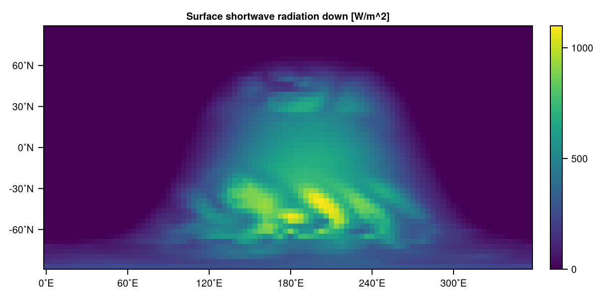

osr = simulation.variables.parameterizations.outgoing_shortwave
heatmap(osr,title="Outgoing shortwave radiation [W/m^2]")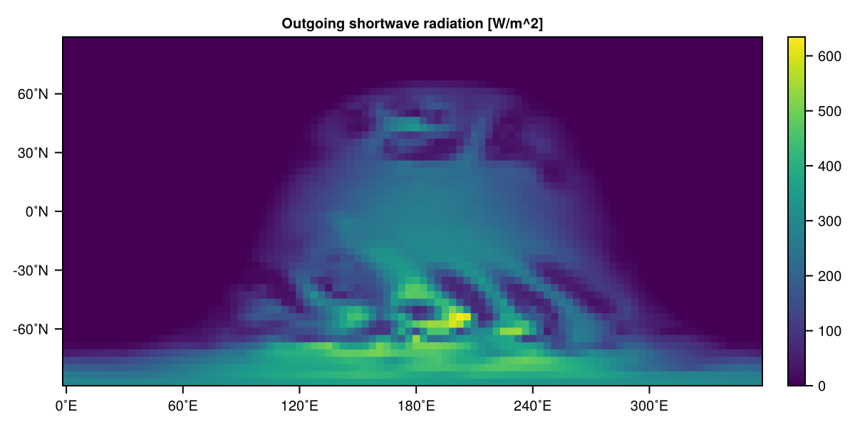

For dry models (no water vapor or clouds):

Use OneBandGreyShortwave instead, which automatically uses NoClouds and TransparentShortwaveTransmissivity:

using SpeedyWeather, CairoMakie
spectral_grid = SpectralGrid(truncation=32, nlayers=8)
model = PrimitiveDryModel(spectral_grid; shortwave_radiation=OneBandGreyShortwave(spectral_grid))
simulation = initialize!(model)
run!(simulation, period=Week(1))

# The shortwave fluxes can be visualised
ssrd = simulation.variables.parameterizations.surface_shortwave_down
heatmap(ssrd, title="Surface shortwave radiation (dry model) [W/m^2]")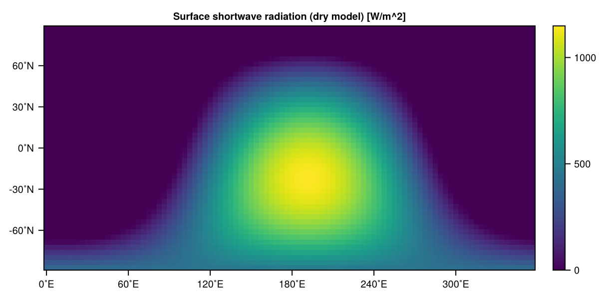

Parameterization options

The OneBandShortwave scheme includes several configurable components:

Cloud schemes

The cloud scheme can be specified when constructing the radiation scheme:

• DiagnosticClouds(spectral_grid) (default): Diagnoses clouds from humidity and precipitation

• NoClouds(spectral_grid): No clouds (used in OneBandGreyShortwave)

Transmissivity schemes

The atmospheric transmissivity can be calculated using:

• BackgroundShortwaveTransmissivity(spectral_grid) (default): Fortran SPEEDY-based transmissivity with zenith correction and absorption by aerosols, water vapor, and clouds

• TransparentShortwaveTransmissivity(spectral_grid): Transparent atmosphere (used in OneBandGreyShortwave)

BackgroundShortwaveTransmissivity

For each layer , the transmissivity is

with

•     (zenith-path correction; is the zenith angle)

•    from the half-levels in the grid geometry

• the column surface pressure

• dry-air absorptivity (absorptivity_dry_air)

• aerosol absorptivity (absorptivity_aerosol), scaled by when aerosols = true

• water-vapor absorptivity (absorptivity_water_vapor) times specific humidity

•   cloud absorptivity added below the diagnosed cloud top, scaled by cloud cover

All absorptivity coefficients are per Pa. The resulting values are computed once per column and reused for both the downward and upward sweeps in OneBandShortwaveRadiativeTransfer.

TransparentShortwaveTransmissivity details

Sets   for all layers and bands, effectively skipping atmospheric attenuation while still computing surface and cloud reflections in the radiative transfer step.

Stratocumulus clouds

The DiagnosticClouds scheme includes a use_stratocumulus flag (default: true) that enables the diagnostic stratocumulus cloud parameterization over oceans:

using SpeedyWeather, CairoMakie

spectral_grid = SpectralGrid()
sw_no_sc = OneBandShortwave(spectral_grid, clouds = DiagnosticClouds(spectral_grid; use_stratocumulus=false))

model = PrimitiveWetModel(spectral_grid; shortwave_radiation=sw_no_sc)
sim = initialize!(model)
run!(sim, period=Day(5))
ssrd = sim.variables.parameterizations.surface_shortwave_down
heatmap(ssrd, title="No stratocumulus clouds [W/m^2]")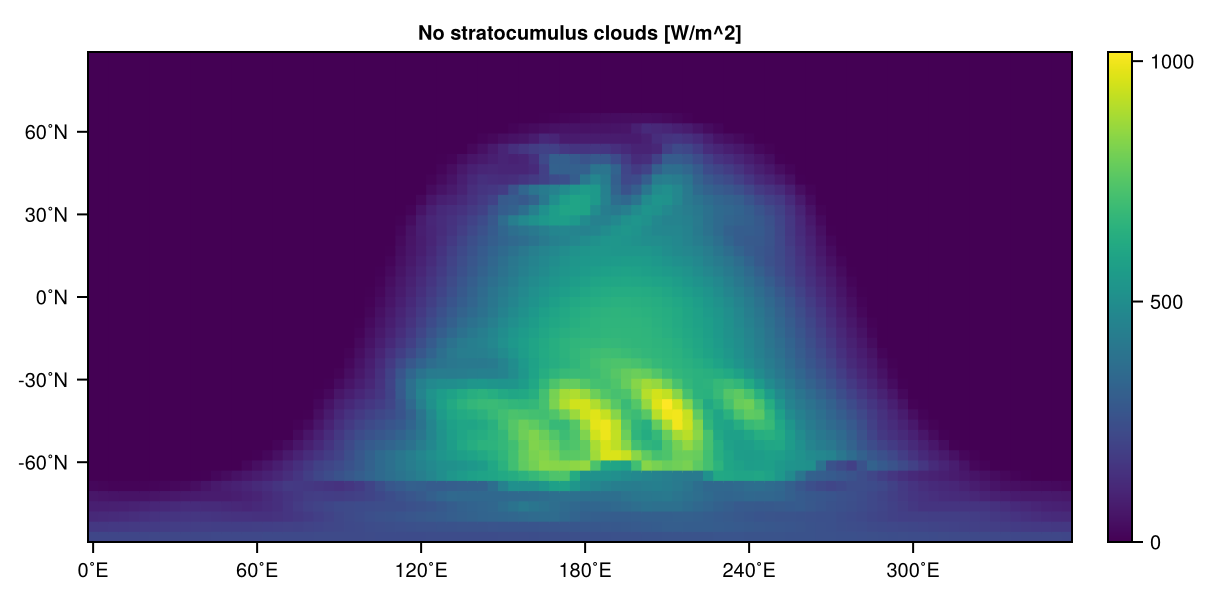

Greenhouse gases

Greenhouse gas concentrations can be prescribed as time-varying scalar quantities and are tracked as prognostic variables. For example, an ExponentialCO2 concentration is fitted to the Keeling curve. To customise or add greenhouse gases, pass a NamedTuple of gas objects to greenhouse_gases. The key of the named tuple will be used for the variable name, so co2 = ..., carbon_dioxide = ... can co-exist.

spectral_grid = SpectralGrid(truncation=32, nlayers=8)

# constant CO2 at 420 ppm
model = PrimitiveWetModel(spectral_grid; greenhouse_gases = (; co2 = CO2(spectral_grid, 420)))
simulation = initialize!(model)
simulation.variables.prognostic.greenhouse_gases.co2[]

420.0f0

A CO2 concentration that increases exponentially over time:

co2 = ExponentialCO2(spectral_grid)

ExponentialCO2{Float32, DateTime} <: SpeedyWeather.AbstractCO2
├ base_concentration::Float32 = 280.0
├ start::DateTime = 1850-01-01T00:00:00
├ a::Float32 = 3.85
└ b::Float32 = 0.020833334

Step-change scenarios are also available: TwoTimesCO2 and FourTimesCO2 double or quadruple the preindustrial CO2 at a given date (default: year 2000). Any callable f(t::DateTime) -> concentration_in_ppm can be wrapped in CO2(f) for a fully custom trajectory.

Radiation schemes not yet CO2-aware

The greenhouse gas concentrations are tracked as prognostic variables and evolve correctly in time, but the radiation schemes (OneBandLongwave etc.) have not yet been updated to use them. Changing CO2 therefore has no effect on the radiative fluxes or temperature tendencies at this stage. This is work in progress.

References

[^PG06]: Paulius and Garner, 2006. JAS. DOI:10.1175/JAS3705.1

[^SW23]: Seeley, J. T. & Wordsworth, R. D. Moist Convection Is Most Vigorous at Intermediate Atmospheric Humidity. Planet. Sci. J. 4, 34 (2023). DOI:10.3847/PSJ/acb0cb

[^JZ22]: Jeevanjee, N. & Zhou, L. On the Resolution‐Dependence of Anvil Cloud Fraction and Precipitation Efficiency in Radiative‐Convective Equilibrium. J Adv Model Earth Syst 14, e2021MS002759 (2022). DOI:10.1029/2021MS002759

[^KMB06]: Kucharski, F., Molteni, F., & Bracco, A. SPEEDY: A simplified atmospheric general circulation model. ICTP, Trieste, Italy. Appendix A: Model Equations and Parameters (2006). PDF

[^FH06]: Frierson DMW, IM Held, P Zurita-Gotor. A Gray-Radiation Aquaplanet Moist GCM. Part I: Static Stability and Eddy Scale (2006). Journal of the Atmospheric Sciences 63:10. DOI: 10.1175/JAS3753.1