Examples 3D

The following showcases several examples of SpeedyWeather.jl simulating the Primitive equations with and without humidity and with and without physical parameterizations.

See also Examples 2D for examples with the Barotropic vorticity equation and the shallow water model.

Jablonowski-Williamson baroclinic wave

using SpeedyWeather
spectral_grid = SpectralGrid(trunc = 31, nlayers = 8, Grid=FullGaussianGrid, dealiasing = 3)

orography = ZonalRidge(spectral_grid)
initial_conditions = (;                             # collect initial conditions into NamedTuple (keys don't matter)
    vordiv = ZonalWind(spectral_grid),
    temperature = JablonowskiTemperature(spectral_grid),
    pressure = ConstantPressure(spectral_grid))

model = PrimitiveDryModel(spectral_grid; orography, initial_conditions, dynamics_only = true)
simulation = initialize!(model)
run!(simulation, period = Day(9))

The Jablonowski-Williamson baroclinic wave test case[^JW06] using the Primitive equation model particularly the dry model, as we switch off all parameterizations (and ocean, sea_ice and land) with dynamics_only = true. We want to use 8 vertical levels, and a lower resolution of T31 on a [full Gaussian grid](@ref FullGaussianGrid). The Jablonowski-Williamson initial conditions areZonalWindfor vorticity and divergence (curl and divergence ofu, v),JablonowskiTemperaturefor temperature andZeroInitiallyfor pressure. The orography is just aZonalRidge. There is no forcing and the initial conditions are baroclinically unstable which kicks off a wave propagating eastward. This wave becomes obvious when visualised with

using CairoMakie

vor = simulation.variables.grid.vorticity[:, end]
heatmap(vor, title="Surface relative vorticity")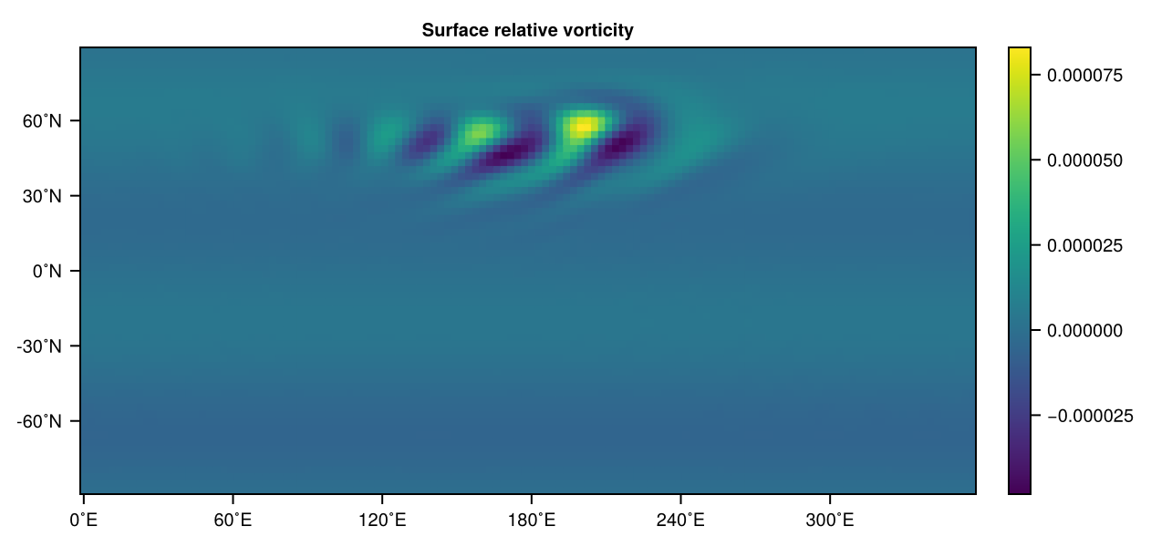

Held-Suarez forcing

using SpeedyWeather
spectral_grid = SpectralGrid(trunc = 31, nlayers = 8)

# construct model with only Held-Suarez forcing, no other physics
model = PrimitiveDryModel(
    spectral_grid,

    # Held-Suarez forcing and drag
    forcing = HeldSuarez(spectral_grid),
    drag = LinearDrag(spectral_grid),

    # switch off other parameterizations, ocean, sea ice and land
    dynamics_only = true,

    # use Earth's orography
    orography = EarthOrography(spectral_grid)
)

simulation = initialize!(model)
run!(simulation, period = Day(20))

The code above defines the Held-Suarez forcing [^HS94] in terms of temperature relaxation and a linear drag term that is applied near the planetary boundary but switches off all other parameterizations in the primitive equation model without humidity. One could also just switch off the boundary layer scheme which would also automatically turn off the surface fluxes (heat and momentum) as they aren't supposed to run with Held-Suarez forcing. But to also avoid the calculation being run at all we use dynamics_only = true. The forcing and drag are considered to be terms of the dynamical core (regardless of which process they represent conceptually). Generally, model components can just be set to nothing where intuitive.

Visualising surface temperature with

using CairoMakie

temp = simulation.variables.grid.temperature[:, end]
heatmap(temp, title="Surface temperature [K]", colormap=:thermal)

Aquaplanet

using SpeedyWeather

# components
spectral_grid = SpectralGrid(trunc=31, nlayers=8)
ocean = AquaPlanet(spectral_grid, temp_equator=302, temp_poles=273)
land_sea_mask = AquaPlanetMask(spectral_grid)
orography = NoOrography(spectral_grid)

# create model, initialize, run
model = PrimitiveWetModel(spectral_grid; ocean, land_sea_mask, orography)
simulation = initialize!(model)
run!(simulation, period=Day(20))

Here we have defined an aquaplanet simulation by

• creating an ocean::AquaPlanet. This will use constant sea surface temperatures that only vary with latitude (and not with time).

• creating a land_sea_mask::AquaPlanetMask this will use a land-sea mask with false=ocean everywhere.

• creating an orography::NoOrography which will have no orography and zero surface geopotential.

All passed on to the model constructor for a PrimitiveWetModel, we have now a model with humidity and physics parameterization as they are defined by default (typing model will give you an overview of its components). We could have change the model.land and model.vegetation components too, but given the land-sea masks masks those contributions to the surface fluxes anyway, this is not necessary. Note that neither sea surface temperature, land-sea mask or orography have to agree. It is possible to have an ocean on top of a mountain. For an ocean grid-cell that is (partially) masked by the land-sea mask, its value will be (fractionally) ignored in the calculation of surface fluxes (potentially leading to a zero flux depending on land surface temperatures).

Now with the following we visualize the surface humidity after the 50 days of simulation. We use 50 days as without mountains it takes longer for the initial conditions to become unstable. The surface humidity shows small-scale patches in the tropics, which is a result of the convection scheme, causing updrafts and downdrafts in both humidity and temperature.

using CairoMakie

humid = simulation.variables.grid.humidity[:, end]
heatmap(humid, title="Surface specific humidity [kg/kg]", colormap=:oslo)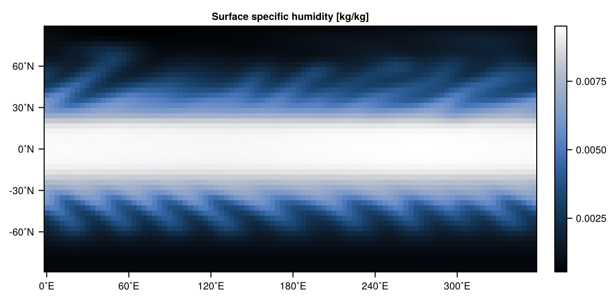

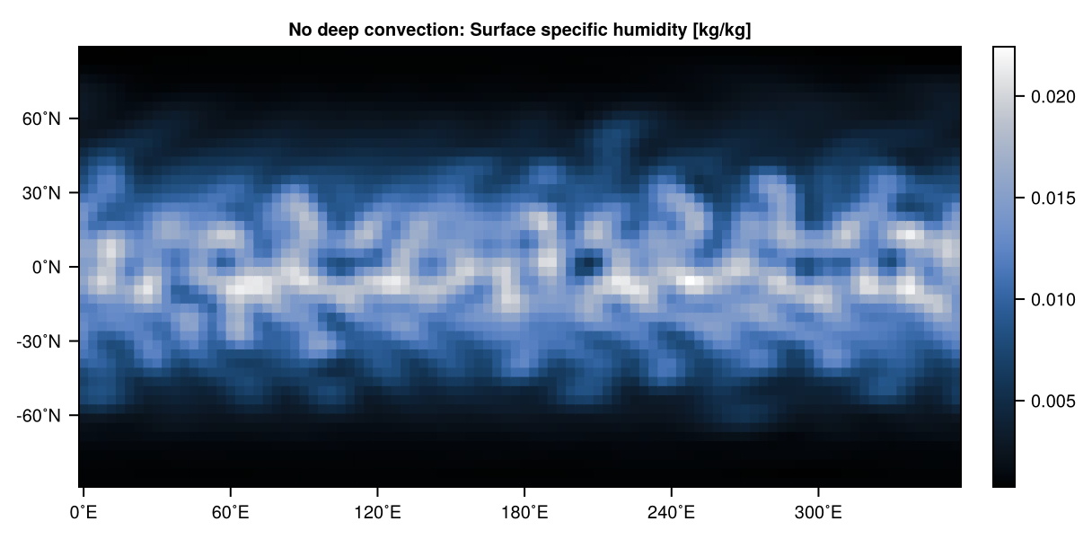
Aquaplanet without (deep) convection

Now we want to compare the previous simulation to a simulation without deep convection, called BettsMillerDryConvection, because it is the Betts-Miller convection but with humidity set to zero in which case the convection is always non-precipitating shallow (because the missing latent heat release from condensation makes it shallower) convection. In fact, this convection is the default when using the PrimitiveDryModel. Instead of redefining the Aquaplanet setup again, we simply reuse these components spectral_grid, ocean, land_sea_mask and orography (because spectral_grid hasn't changed this is possible).

# Execute the code from Aquaplanet above first!
convection = BettsMillerDryConvection(spectral_grid, time_scale=Hour(4))

# reuse other model components from before
model = PrimitiveWetModel(spectral_grid; ocean, land_sea_mask, orography, convection)

simulation = initialize!(model)
run!(simulation, period=Day(20))

humid = simulation.variables.grid.humidity[:, end]
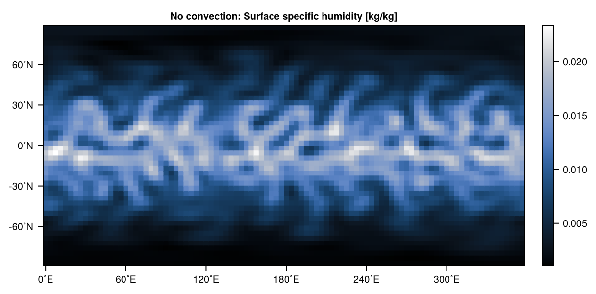
heatmap(humid, title="No deep convection: Surface specific humidity [kg/kg]", colormap=:oslo)

But we also want to compare this to a setup where convection is completely disabled, i.e. convection = nothing

# Execute the code from Aquaplanet above first!
convection = nothing

# reuse other model components from before
model = PrimitiveWetModel(spectral_grid; ocean, land_sea_mask, orography, convection)

simulation = initialize!(model)
run!(simulation, period=Day(20))

humid = simulation.variables.grid.humidity[:, end]
heatmap(humid, title="No convection: Surface specific humidity [kg/kg]", colormap=:oslo)

And the comparison looks like

Large-scale vs convective precipitation

using SpeedyWeather

# components
spectral_grid = SpectralGrid(trunc = 31, nlayers = 8)
large_scale_condensation = ImplicitCondensation(spectral_grid, snow = false)
convection = BettsMillerConvection(spectral_grid)

# create model, initialize, run
model = PrimitiveWetModel(spectral_grid; large_scale_condensation, convection)
simulation = initialize!(model)
run!(simulation, period = Day(10))

We run the default PrimitiveWetModel with ImplicitCondensation as large-scale condensation (see Implicit large-scale condensation) and the BettsMillerConvection for convection (see Simplified Betts-Miller). These schemes have some additional parameters, we leave them as default for now, but you could do ImplicitCondensation(spectral_grid, relative_humidity_threshold = 0.8) to let it rain at 80% instead of 100% relative humidity. We now want to analyse the precipitation that comes from these parameterizations.

Note that the following only considers liquid precipitation for simplicity. We set snow = false in ImplicitCondensation and therefore deal with rain only.

using CairoMakie

(; rain_large_scale, rain_convection) = simulation.variables.parameterizations
m2mm = 1000     # convert from [m] to [mm]
heatmap(m2mm*rain_large_scale, title="Large-scale precipiation (rain) [mm]: Accumulated over 10 days", colormap=:dense)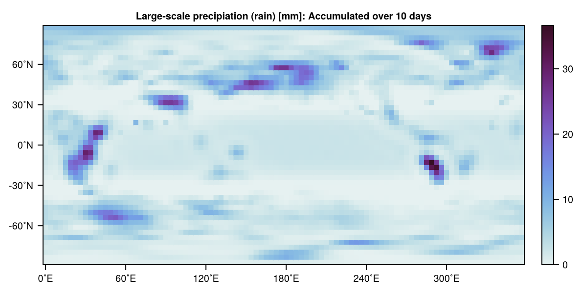

Precipitation (rain, both large-scale and convective) are written into the simulation.variables.parameterizations which, however, accumulate all precipitation during simulation. In the NetCDF output, precipitation rate (in mm/hr) is calculated from accumulated precipitation as a post-processing step. More interactively, you can also reset these accumulators and integrate for another 6 hours to get the precipitation only in that period.

# reset accumulators and simulate 6 hours
simulation.variables.parameterizations.rain_large_scale .= 0
simulation.variables.parameterizations.rain_convection .= 0
run!(simulation, period=Hour(6))

# visualise, rain_* arrays are flat copies, no need to read them out again!
m2mm_hr = (1000*Hour(1)/Hour(6))    # convert from [m] to [mm/hr]
heatmap(m2mm_hr*rain_large_scale, title="Large-scale precipiation (rain) [mm/hr]", colormap=:dense)
heatmap(m2mm_hr*rain_convection, title="Convective precipiation (rain) [mm/hr]", colormap=:dense)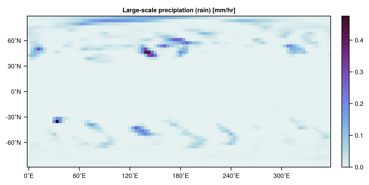

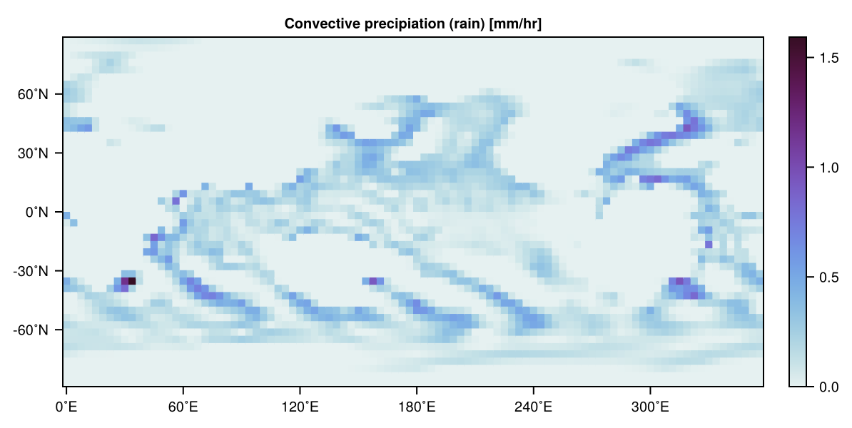
As the precipitation fields are accumulated meters over the integration period we divide by 6 hours to get a precipitation rate but then multiply with 1 hour and 1000 to get the typical precipitation unit of .

References

[^JW06]: Jablonowski, C. and Williamson, D.L. (2006), A baroclinic instability test case for atmospheric model dynamical cores. Q.J.R. Meteorol. Soc., 132: 2943-2975. DOI:10.1256/qj.06.12

[^HS94]: Held, I. M. & Suarez, M. J. A Proposal for the Intercomparison of the Dynamical Cores of Atmospheric General Circulation Models. Bulletin of the American Meteorological Society 75, 1825-1830 (1994). DOI:10.1175/1520-0477(1994)075<1825:APFTIO>2.0.CO;2