Particle advection

All SpeedyWeather.jl models support particle advection. Particles are objects without mass or volume at a location   (longitude , latitude , vertical sigma coordinate , see Sigma coordinates) that are moved with the wind at that location. The location of the -th particle changes as follows

This equation applies in 2D, i.e.   and   or in 3D, i.e.   and   with the vertical velocity in coordinates. Both are supported, selected via ParticleAdvection2D or ParticleAdvection3D respectively, see 3D particle advection below. With ParticleAdvection2D in the Primitive equation model the vertical layer on which the advection takes place is chosen with the layer keyword (default layer = 1, the topmost layer). Particles are therefore not advected with the vertical velocity but maintain a constant pressure ratio compared to the surface pressure ( is constant). (See also Tracer advection for advecting continuous fields instead of individual particles.)

Discretization of particle advection

The particle advection equation has to be discretized to be numerically solved. While the particle location can generally be anywhere on the sphere, the velocity is only available on the discrete grid points of the simulation, such that requires an interpolation in order to obtain a velocity at the particles location to move it around. Dropping the subscript in favour a subscript denoting the time step, with Euler forward the equation can be discretized as

Meaning we have used the velocity field at both departure time and departure location to update a particle's location which makes this scheme first order accurate. But only a single interpolation of the velocity field, which, in fact, is one per dimension, is necessary. Note that the time step here and the time step to solve the dynamics do not have to be identical. We could use a larger time step for the particle advection then to solve the dynamics inside the model, and because the stability criteria for these equations are different, one is encouraged to do so. Also because the particles are considered passive, meaning that their location does not influence the other prognostic variables.

We can write down a more accurate scheme at the cost of a second interpolation step. The Heun method, also called predictor-corrector is 2nd order accurate and uses an average of the velocity at departure time and location and at a (predicted meaning preliminary) arrival point and arrival time  .

Because we don't have available at time , we perform this integration retrospectively, i.e. if the other model dynamics have reached time   then we let the particle advection catch up by integrating them from to  . This, however, requires some storage of the velocity at the previous advection time step. Remember that this does not need to be the time step for the momentum equations and could be much further in the past. We could either store as a grid-point field or only its interpolated values. In the case of fewer particles than grid points the latter is more efficient and this is also what we do in SpeedyWeather. Let square brackets   denote an interpolation then we perform the interpolation that's required to step from to   already on the time step that goes from   to .

Denoted here as the last line with the left-hand side becoming the last term of the first line in the next time step    . Now it becomes clearer that there are two interpolations required on every time step.

We use for horizontal coordinates degrees, such that we need to scale the time step with (radius ) for advection in latitude and with for advection in longitude (because the distance between meridians decreases towards the poles). We move the division by the radius conveniently into the time step as are also the momentum equations scaled with the radius, see Radius scaling.

Technically, a particle moved with a given velocity follows a great circle in spherical coordinates. This means that

becomes a bad approximation when the time step and or the velocity are large. However, for simplicity and to avoid the calculation of the great circle we currently do use this to move particles with a given velocity. We essentially assume a local cartesian coordinate system instead of the geodesics in spherical coordinates. However, for typical time steps of 1 hour and velocities not exceeding 100 m/s the error is not catastrophic and can be reduced with a shorter time step. We may switch to great circle calculations in future versions.

Create a particle

So much about the theory

A Particle at location 10˚E and 30˚N (and  ) can be created as follows,

using SpeedyWeather
p = Particle(lon=10, lat=30, σ=0)
p = Particle(lon=10, lat=30)
p = Particle(10, 30, 0)
p = Particle(10, 30)

Particle{Float32}(  active,  10.00˚E,  30.00˚N, σ = 0.00)

All of the above are equivalent. Unless a keyword argument is used, longitude is the first argument, followed by latitude (necessary), followed by (can be omitted). Longitudes can be -180˚E to 180˚E or 0 to 360˚E, latitudes have to be -90˚N to 90˚N. You can create a particle with coordinates outside of these ranges (and no error or warning is thrown) but during particle advection they will be wrapped into [0, 360˚E] and [-90˚N, 90˚N], using the mod(::Particle) function, which is similar to the modulo operator but with the second argument hardcoded to the coordinate ranges from above, e.g.

mod(Particle(lon=-30, lat=0))

Particle{Float32}(  active, 330.00˚E,   0.00˚N, σ = 0.00)

which also takes into account pole crossings which adds 180˚ in longitude

mod(Particle(lon=0, lat=100))

Particle{Float32}(  active, 180.00˚E,  80.00˚N, σ = 0.00)

as if the particle has moved across the pole. That way all real values for longitude and latitude are wrapped into the reference range [0, 360˚E] and [-90˚N, 90˚N].

Particles are immutable

Particles are implemented as immutable struct, meaning you cannot change their position by particle.lon = value. You have to think of them as integers or floats instead. If you have a particle p and you want to change its position to the Equator for example you need to create a new one new_particle = Particle(p.lon, 0, p.σ).

By default Float32 is used, but providing coordinates in Float64 will promote the type accordingly. Also by default, particles are active which is indicated by the field active of Particle, a boolean. Active particles are moved following the equation above, but inactive particles are not. You can activate or deactivate a particle like so

deactivate(p)

Particle{Float32}(inactive,  10.00˚E,  30.00˚N, σ = 0.00)

and so

activate(p)

Particle{Float32}(  active,  10.00˚E,  30.00˚N, σ = 0.00)

or check its activity by isactive(::Particle) returning true or false. The zero-element of the Particle type is

zero(Particle)

Particle{Float32}(  active,   0.00˚E,   0.00˚N, σ = 0.00)

and you can also create a random particle which uses a raised cosine distribution in latitude for an equal area-weighted uniform distribution over the sphere

rand(Particle{Float32})         # specify number format
rand(Particle)                  # or not (defaults used instead)

Particle{Float32}(  active,  75.84˚E,  21.55˚N, σ = 0.93)

Advecting particles

The Particle type can be used inside vectors, e.g.

zeros(Particle{Float32}, 3)
rand(Particle{Float64}, 5)

5-element Vector{Particle{Float64}}:
 Particle{Float64}(  active, 176.66˚E,  31.88˚N, σ = 0.78)
 Particle{Float64}(  active,  74.46˚E,  29.44˚N, σ = 0.93)
 Particle{Float64}(  active, 345.87˚E, -27.46˚N, σ = 0.74)
 Particle{Float64}(  active, 273.87˚E,  42.89˚N, σ = 0.08)
 Particle{Float64}(  active, 228.97˚E,  75.29˚N, σ = 0.94)

which is how particles are represented inside a SpeedyWeather Simulation. Note that the default initial state of particles is active. In SpeedyWeather all particles can be activated or deactivated at any time using the activate and deactivate functions.

We create a ParticleAdvection2D with the nparticles keyword to determine the number of particles (use the layer keyword for 3D models)

spectral_grid = SpectralGrid(nlayers = 1)
particle_advection = ParticleAdvection2D(spectral_grid, nparticles = 3)
model = BarotropicModel(spectral_grid; particle_advection)
simulation = initialize!(model)

Simulation{...} (740.94 KB)
├ variables::Variables{...} (139.95 KB)
└ model::BarotropicModel{...} (621.47 KB)

Then the particles live as AbstractVector{Particle} inside the variables

vars = simulation.variables     # for brevity
vars.prognostic.particles

3-element Vector{Particle{Float32}}:
 Particle{Float32}(  active, 174.14˚E,   3.10˚N, σ = 0.37)
 Particle{Float32}(  active, 287.99˚E,   8.85˚N, σ = 0.90)
 Particle{Float32}(  active, 113.34˚E,  -3.94˚N, σ = 0.66)

Which are placed in random locations (using rand) initially. In order to change these (e.g. to set the initial conditions) you can do

vars.prognostic.particles[1] = Particle(lon=-120, lat=45)
vars.prognostic.particles

3-element Vector{Particle{Float32}}:
 Particle{Float32}(  active, -120.00˚E,  45.00˚N, σ = 0.00)
 Particle{Float32}(  active, 287.99˚E,   8.85˚N, σ = 0.90)
 Particle{Float32}(  active, 113.34˚E,  -3.94˚N, σ = 0.66)

which sets the first particle (you can think of the index as the particle identification) to some specified location, or you could deactivate a particle with

first_particle = vars.prognostic.particles[1]
vars.prognostic.particles[1] = deactivate(first_particle)
vars.prognostic.particles

3-element Vector{Particle{Float32}}:
 Particle{Float32}(inactive, -120.00˚E,  45.00˚N, σ = 0.00)
 Particle{Float32}(  active, 287.99˚E,   8.85˚N, σ = 0.90)
 Particle{Float32}(  active, 113.34˚E,  -3.94˚N, σ = 0.66)

After 10 days of simulation the particle locations have changed

run!(simulation, period=Day(10))
simulation.variables.particles.locations

3-element Vector{Particle{Float32}}:
 Particle{Float32}(  active,   0.00˚E,   0.00˚N, σ = 0.00)
 Particle{Float32}(  active, 337.72˚E,   8.16˚N, σ = 0.50)
 Particle{Float32}(  active,  85.06˚E,  -5.28˚N, σ = 0.50)

Woohoo! We just advected some particles. Note that the active particles have their vertical coordinate set to value of the layer they are being advected on given that we defined ParticleAdvection2D with layer = 1 as default (which has that coordinate value as default).

3D particle advection

In addition to being advected horizontally on a fixed model layer (ParticleAdvection2D), particles can also be advected freely in the vertical (ParticleAdvection3D). Instead of keeping fixed, a particle's coordinate now evolves in time too, driven by the model's (diagnostic) vertical velocity, in exactly the same way as longitude and latitude evolve with and . As in the horizontal, the radius scaling is moved into the time step: the model stores the vertical velocity as   (radius-scaled like vorticity and divergence, see Radius scaling), so a particle moves by  . This is currently only available for the Primitive equation models (PrimitiveDryModel, PrimitiveWetModel) as it requires a vertically-resolved, diagnosed vertical velocity; BarotropicModel and ShallowWaterModel have no such concept and continue to only support ParticleAdvection2D.

Vertical interpolation

Wind is only known on the model's discrete layers so a particle's continuous position has to be translated into a vertical interpolation, similar to how longitude and latitude are translated into the horizontal (4-point "anvil") interpolation described above. This is done in two steps:

1. Find the two neighbouring model layers that bracket the particle's . If the particle is above the topmost or below the bottommost layer, the value on that layer is used instead of extrapolating beyond it.

2. Interpolate horizontally onto each of these two layers separately, using exactly the same 4-point anvil interpolation as for ParticleAdvection2D, then linearly blend the two resulting values by how far the particle's lies between the two layers.

In short, 3D interpolation is the same horizontal interpolation done twice (once per bracketing layer) and then blended vertically. Near the poles, where the anvil stencil has no meaningful neighbours, the same ring-average substitute as for the 2D case is used, just computed once for every model layer instead of once for a single 2D field.

Flexibility and limitations: horizontal precompute versus vertical on the fly

The horizontal and vertical directions are treated quite differently for performance reasons. Locating a particle within the horizontal grid (RingGrids.update_locator!) is relatively expensive, it searches through the rings of latitude and, within a ring, through its longitudes, so it is computed once for every new horizontal position of the particles, i.e. twice per advection step (at the predicted and at the corrected position of Heun's method), and the resulting grid indices and interpolation weights are reused for all fields interpolated at that position (, and ). Locating a particle's vertical bracket, on the other hand, is cheap: a short scan through as few as a handful of layers, so it is simply recomputed on the fly every time a value is interpolated, with no separate precompute or storage step.

This is a deliberate trade-off that assumes there are many fewer vertical layers than horizontal grid points, typically true (e.g. 8 vertical layers against many thousands of horizontal grid points). Some consequences:

• Increasing the vertical resolution (nlayers) adds essentially no cost or storage to particle advection beyond the layer vector the model already needs, plus two small per-layer pole-average buffers (see RingGrids.AnvilLocator).

• Because the same horizontal indices and weights are reused for both bracketing layers, horizontal and vertical location are decoupled: the (horizontal) locator does not depend on and is reused for all layers and for fields on full and half layers alike.

• Above the topmost and below the bottommost full layer, and are taken from that layer rather than extrapolated. The particle's itself is not held there: it keeps moving with , which lives on the half layers spanning the whole column    and vanishes at   and  . Together with being clamped to after every step, particles therefore cannot leave the atmosphere through the model top or fall through the surface.

Interface example

Using ParticleAdvection3D instead of ParticleAdvection2D is enough to switch a simulation from 2D to 3D particle advection; there is no layer keyword any more as particles are free to move to any layer

using SpeedyWeather
spectral_grid = SpectralGrid(nlayers = 8)
particle_advection = ParticleAdvection3D(spectral_grid, nparticles = 3)
model = PrimitiveDryModel(spectral_grid; particle_advection)
simulation = initialize!(model)
run!(simulation, period = Day(2))
simulation.variables.prognostic.particles

3-element Vector{Particle{Float32}}:
 Particle{Float32}(  active, 291.61˚E,  10.42˚N, σ = 0.41)
 Particle{Float32}(  active, 296.92˚E, -83.93˚N, σ = 0.04)
 Particle{Float32}(  active,  78.84˚E, -20.85˚N, σ = 0.82)

Every particle's σ field is now updated over time, whereas with ParticleAdvection2D it would have remained fixed at the layer-th value of model.geometry.σ_layers_full.

To check that the vertical trajectories are smooth and reasonable we can track the particles with a ParticleTracker (see Tracking particles below), which also writes out , and plot every particle's over time

particle_tracker = ParticleTracker(spectral_grid, schedule = Schedule(every = Hour(4)))
particle_advection = ParticleAdvection3D(spectral_grid, nparticles = 20, every_n_time_steps = 6)
model = PrimitiveWetModel(spectral_grid; particle_advection)
add!(model.callbacks, particle_tracker)
simulation = initialize!(model)
run!(simulation, period = Day(10))

using NCDatasets, CairoMakie
ds = NCDataset(joinpath(model.output.run_folder, particle_tracker.filename))
σ = ds["sigma"][:, :]
hours = ds["time"].var[:]      # raw hours since start, not decoded into DateTime
close(ds)

fig = Figure()
ax = Axis(fig[1, 1], xlabel = "time [hours]", ylabel = "σ", yreversed = true)
[lines!(ax, hours, σ[i, :]) for i in axes(σ, 1)]

[ Info: ParticleTracker{Vector{Float32}} callback added with key callback_KdUo
[ Info: ParticleTracker writes to particles.nc as output=false

with yreversed = true so that the surface ( ) is at the bottom. We use every_n_time_steps = 6 here (default) to advect the particles less frequently than the model time step. If the tracker time step (here 4 hours) is not a multiple of the particle advection time step the output may look staircase-like, adjust accordingly.

Tracking particles

A ParticleTracker is implemented as a callback, see Callbacks, outputting the particle locations via netCDF. We can create it like

using SpeedyWeather
spectral_grid = SpectralGrid(nlayers = 1)
particle_tracker = ParticleTracker(spectral_grid, schedule = Schedule(every = Hour(3)))

ParticleTracker{Vector{Float32}} <: SpeedyWeather.AbstractCallback
├ schedule::Schedule = Schedule <: SpeedyWeather.AbstractSchedule
├...
├ filename::String = particles.nc
├ path::String = 
├ compression_level::Int64 = 1
├ shuffle::Bool = false
├ keepbits::Int64 = 15
├ nparticles::Int64 = 0
├ netcdf_file::Nothing = nothing
└ arrays: lon, lat, σ

which would output every 3 hours (the default). This output frequency might be slightly adjusted depending on the time step of the dynamics to output every n time steps (an @info is thrown if that is the case), see Schedules. Further options on compression are available as keyword arguments ParticleTracker(spectral_grid, keepbits=15) for example. The callback is then added after the model is created

particle_advection = ParticleAdvection2D(spectral_grid, nparticles = 100)
model = ShallowWaterModel(spectral_grid; particle_advection)
add!(model.callbacks, particle_tracker)

Dict{Symbol, SpeedyWeather.AbstractCallback} with 1 entry:
  :callback_CBC5 => ParticleTracker{Vector{Float32}} <: SpeedyWeather.AbstractC…

which will give it a random key too in case you need to remove it again (more on this in Callbacks). If you now run the simulation the particle tracker is called on particle_tracker.every_n_time_steps and it continuously writes into particle_tracker.netcdf_file which is placed in the run folder similar to other NetCDF output. For example, the run folder can be obtained after the simulation by model.output.run_folder.

simulation = initialize!(model)
run!(simulation, period = Day(10))
model.output.run_folder

""

As we don't have output = true, by default, the particles.nc file will be written the to current working directory. You can read the netCDF file with

using NCDatasets
run_folder = model.output.run_folder                    # if output = true the run_???? string with run number
path = joinpath(run_folder, particle_tracker.filename)  # "particles.nc" by default if output = false
ds = NCDataset(path)
ds["lon"]
ds["lat"]

lat (100 × 91)
  Datatype:    Float32 (Float32)
  Dimensions:  particle × time
  Attributes:
   units                = degrees_east
   long_name            = latitude

where the last two lines are lazy loading a matrix with each row a particle and each column a time step. You may do ds["lon"][:,:] to obtain the full Matrix. We had specified spectral_grid.nparticles above and we will have time steps in this file depending on the period the simulation ran for and the particle_tracker.Δt output frequency. We can visualise the particles' trajectories with

lon = ds["lon"][:,:]
lat = ds["lat"][:,:]
nparticles = size(lon,1)

using CairoMakie
fig = lines(lon[1, :], lat[1, :])                               # first particle only
[lines!(fig.axis, lon[i,:], lat[i,:]) for i in 2:nparticles]   # add lines for other particles

# display updated figure
fig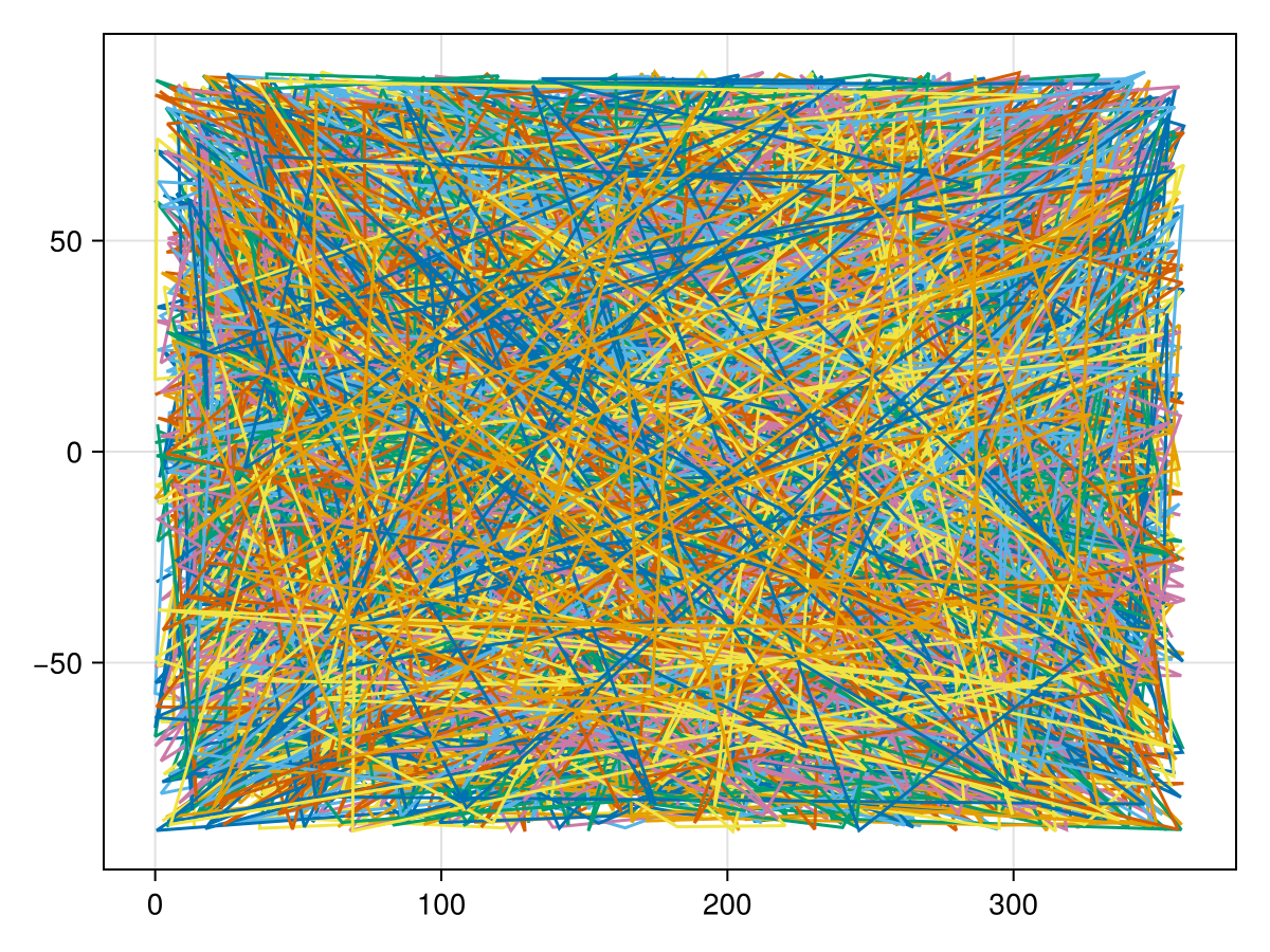

Instead of providing a polished example with a nice projection we decided to keep it simple here because this is probably how you will first look at your data too. As you can see, some particles in the Northern Hemisphere have been advected with a zonal jet and perform some wavy motions as the jet does too. However, there are also some horizontal lines which are automatically plotted when a particles travels across the prime meridian 0˚E = 360˚E. Ideally you would want to use a more advanced projection and plot the particle trajectories as geodetics.

With GeoMakie.jl you can do

using GeoMakie, CairoMakie

fig = Figure()
ga = GeoAxis(fig[1, 1]; dest = "+proj=ortho +lon_0=45 +lat_0=45")
[lines!(ga, lon[i,:], lat[i,:]) for i in 1:nparticles]
fig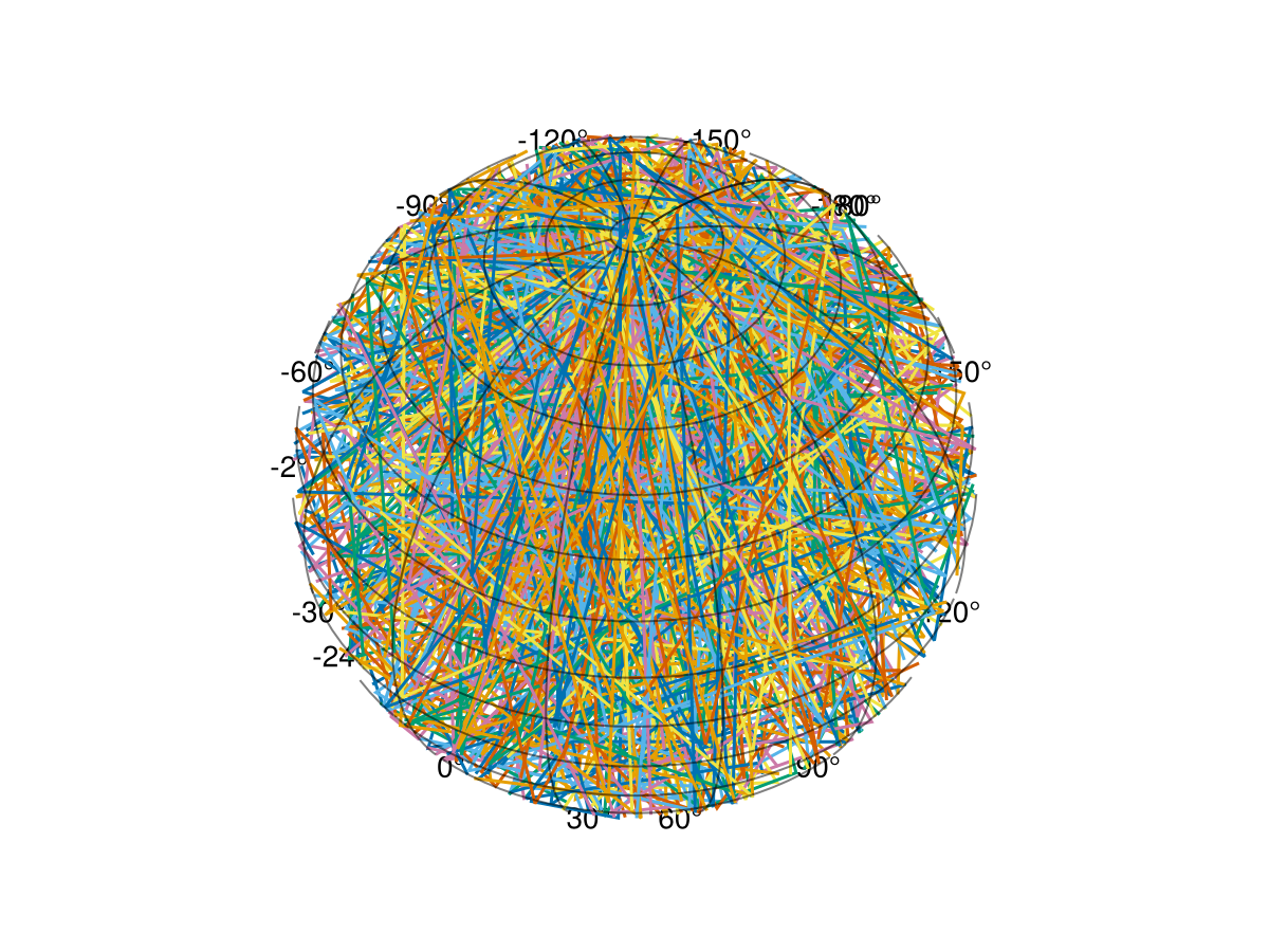

For more advanced visualisations of the particle tracker see the TravellingSailorProblem.jl.