Grids

The spectral transform (the Spherical Harmonic Transform) in SpeedyWeather.jl supports any ring-based equi-longitude grid. Several grids are already implemented but other can be added. The following pages will describe an overview of these grids and but let's start but how they can be used

using SpeedyWeather
spectral_grid = SpectralGrid(Grid = FullGaussianGrid)

SpectralGrid{CPU, Spectrum{...}, FullGaussianGrid{...}}
├ Number format: Float32
├ Spectral:      T31 LowerTriangularMatrix, 560 harmonics
├ Grid:          48-ring FullGaussianGrid, 4608 grid points
├ Resolution:    2.99°, 333km (at 6371km radius)
├ Vertical:      8-layer atmosphere
└ Architecture:  CPU using Array

The life of every SpeedyWeather.jl simulation starts with a SpectralGrid object which defines the resolution in spectral and in grid-point space. The generator SpectralGrid() can take as a keyword argument Grid which can be any of the grids described below. The resolution of the grid, however, is not directly chosen, but determined from the spectral resolution trunc and the dealiasing factor. More in SpectralGrid and Matching spectral and grid resolution.

RingGrids is a module too!

While RingGrids is the underlying module that SpeedyWeather.jl uses for data structs on the sphere, the module can also be used independently of SpeedyWeather, for example to interpolate between data on different grids. See RingGrids

Ring-based equi-longitude grids

SpeedyWeather.jl's spectral transform supports all ring-based equi-longitude grids. These grids have their grid points located on rings with constant latitude and on these rings the points are equi-spaced in longitude. There is technically no constrain on the spacing of the latitude rings, but the Legendre transform requires a quadrature to map those to spectral space and back. Common choices for latitudes are the Gaussian latitudes which use the Gaussian quadrature, or equi-angle latitudes (i.e. just regular latitudes but excluding the poles) that use the Clenshaw-Curtis quadrature. The longitudes have to be equi-spaced on every ring, which is necessary for the fast Fourier transform, as one would otherwise need to use a non-uniform Fourier transform. In SpeedyWeather.jl the first grid point on any ring can have a longitudinal offset though, for example by spacing 4 points around the globe at 45˚E, 135˚E, 225˚E, and 315˚E. In this case the offset is 45˚E as the first point is not at 0˚E.

Is the FullClenshawGrid a longitude-latitude grid?

Short answer: Yes. The FullClenshawGrid is a specific longitude-latitude grid with equi-angle spacing. The most common grids for geoscientific data use regular spacings for 0-360˚E in longitude and 90˚N-90˚S. The FullClenshawGrid does that too, but it does not have a point on the North or South pole, and the central latitude ring sits exactly on the Equator. We name it Clenshaw following the Clenshaw-Curtis quadrature that is used in the Legendre transfrom in the same way as Gaussian refers to the Gaussian quadrature.

Implemented grids

All grids in SpeedyWeather.jl are a subtype of AbstractGrid, i.e. <: AbstractGrid. We further distinguish between full, and reduced grids. Full grids have the same number of longitude points on every latitude ring (i.e. points converge towards the poles) and reduced grids reduce the number of points towards the poles to have them more evenly spread out across the globe. More evenly does not necessarily mean that a grid is equal-area, meaning that every grid cell covers exactly the same area (although the shape changes).

Currently the following full grids <: AbstractFullGrid are implemented

• FullGaussianGrid, a full grid with Gaussian latitudes

• FullClenshawGrid, a full grid with equi-angle latitudes

and additionally we have FullHEALPixGrid and FullOctaHEALPixGrid which are the full grid equivalents to the HEALPix grid and the OctaHEALPix grid discussed below. Full grid equivalent means that they have the same latitude rings, but no reduction in the number of points per ring towards the poles and no longitude offset. Other implemented reduced grids are

• OctahedralGaussianGrid, a reduced grid with Gaussian latitudes based on an octahedron

• OctahedralClenshawGrid, similar but based on equi-angle latitudes

• HEALPixGrid, an equal-area grid based on a dodecahedron with 12 faces

• OctaHEALPixGrid, an equal-area grid from the class of HEALPix grids but based on an octahedron.

An overview of these grids is visualised here, and a more detailed description follows below.

Visualised are each grid's grid points (white dots) and grid faces (white lines). All grids shown have 16 latitude rings on one hemisphere, Equator included. The total number of grid points is denoted in the top left of every subplot. The sphere is shaded with grey, orange and turquoise regions to denote the hemispheres in a and b, the 8 octahedral faces c, d, f and the 12 dodecahedral faces (or base pixels) in e. Coastlines are added for orientation.

Grid resolution

All grids use the same resolution parameter nlat_half, i.e. the number of rings on one hemisphere, Equator included. The Gaussian grids (full and reduced) do not have a ring on the equator, so their total number of rings nlat is always even and twice nlat_half. Clenshaw-Curtis grids and the HEALPix grids have a ring on the equator such their total number of rings is always odd and one less than the Gaussian grids at the same nlat_half.

HEALPix grids do not use Nside as resolution parameter

The original formulation for HEALPix grids use , the number of grid points along the edges of each basepixel (8 in the figure above), SpeedyWeather.jl uses nlat_half, the number of rings on one hemisphere, Equator included, for all grids. This is done for consistency across grids. We may use for the documentation or within functions though.

Related: Effective grid resolution and Available horizontal resolutions.

Matching spectral and grid resolution

A given spectral resolution can be matched to a variety of grid resolutions. A cubic grid, for example, combines a spectral truncation with a grid resolution (=nlat_half) such that   . Using T31 and an O32 is therefore often abbreviated as Tco31 meaning that the spherical harmonics are truncated at   in combination with N=32, i.e. 64 latitude rings in total on an octahedral Gaussian grid. In SpeedyWeather.jl the choice of the order of truncation is controlled with the dealiasing parameter in the SpectralGrid construction.

Let J be the total number of rings. Then we have

•   for linear truncation, i.e. dealiasing = 1

•   for quadratic truncation, i.e. dealiasing = 2

•   for cubic truncation, , i.e. dealiasing = 3

and in general   for m-th order truncation. So the higher the truncation order the more grid points are used in combination with the same spectral resolution. A higher truncation order therefore makes all grid-point calculations more expensive, but can represent products of terms on the grid (which will have higher wavenumber components) to a higher accuracy as more grid points are available within a given wavelength. Using a sufficiently high truncation is therefore one way to avoid aliasing. A quick overview of how the grid resolution changes when dealiasing is passed onto SpectralGrid on the FullGaussianGrid

trunc	dealiasing	FullGaussianGrid size
31	1	64x32
31	2	96x48
31	3	128x64
42	1	96x48
42	2	128x64
42	3	192x96
...	...	...

You will obtain this information every time you create a SpectralGrid(; Grid, trunc, dealiasing).

Interactively exploring the grids

Based on GeoMakie.jl SpeedyWeather.jl has an extension (meaning only loaded when also using GeoMakie) that defines the globe function which visualises the implemented grids at the desired resolution. With the CairoMakie backend these visualisations are static, but using GLMakie they are interactive. For example

using SpeedyWeather
using GLMakie, GeoMakie

# grid type, resolution parameter nlat_half
globe(FullGaussianGrid, 24)

This will open a window with interactive zoom and rotation, visualising a full Gaussian grid at a resolution of nlat_half = 24 (i.e. 96x48 grid points). You can visualise all grids at a wide range of resolutions for non-interactive plotting use interactive=false, which is also what one should do when using CairoMakie. Additional keyword arguments are coastlines, background among others, check ?globe. You also can visualise data on a grid directly this way which will draw polygons for the cell faces, e.g.

grid = rand(FullGaussianGrid, 24)
globe(grid)

Full Gaussian grid

(called FullGaussianGrid)

using CairoMakie, GeoMakie    # when using GLMakie, use interactive=true (default) for zoom and rotation
globe(FullGaussianGrid, 24, interactive=false)

The full Gaussian grid is a grid that uses regularly spaced longitudes with points that do not reduce in number towards the poles. That means for every latitude the longitudes are

with   the in-ring index (1-based, counting from 0˚ eastward) and the number of longitudinal points on the grid. The first longitude is therefore 0˚, meaning that there is no longitudinal offset on this grid. There are always twice as many points in zonal direction as there are in meridional, i.e.  . The latitudes, however, are not regular, but chosen from the -th zero crossing of the -th Legendre polynomial. For in latitudes

As it can be easy to mix up latitudes, colatitudes and as the Legendre polynomials are defined in an overview of the first Gaussian latitudes (approximated for   for brevity)

	Zero crossings	Latitudes [˚N]
2
4
6

Only even Legendre polynomials are used, such that there is always an even number of latitudes, with no latitude on the Equator. As you can already see from this short table, the Gaussian latitudes do not nest, i.e. different resolutions through different do not share latitudes. The latitudes are also only approximately evenly spaced. Due to the Gaussian latitudes, a spectral transform with a full Gaussian grid is exact as long as the truncation is at least quadratic, see Matching spectral and grid resolution. Exactness here means that only rounding errors occur in the transform, meaning that the transform error is very small compared to other errors in a simulation. This property arises from that property of the Gauss-Legendre quadrature, which is used in the Spherical Harmonic Transform with a full Gaussian grid.

On the full Gaussian grid there are in total grid points, which are squeezed towards the poles, making the grid area smaller and smaller following a cosine. But no points are on the poles as    or is never a zero crossing of the Legendre polynomials.

Octahedral Gaussian grid

(called OctahedralGaussianGrid)

using CairoMakie, GeoMakie    # when using GLMakie, use interactive=true (default) for zoom and rotation
globe(OctahedralGaussianGrid, 24, interactive=false)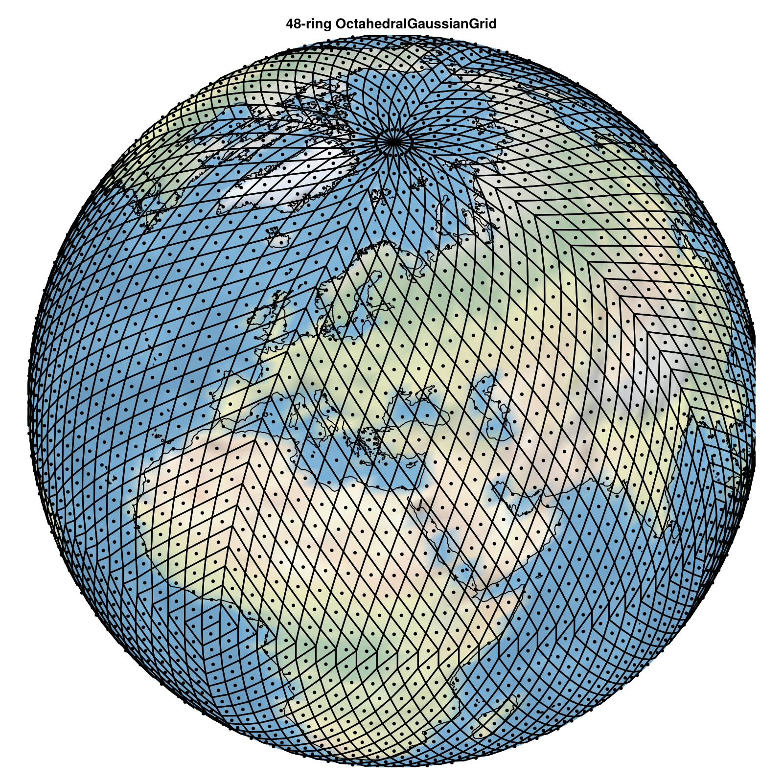

The octahedral Gaussian grid is a reduced grid, i.e. the number of longitudinal points reduces towards the poles. It still uses the Gaussian latitudes from the full Gaussian grid so the exactness property of the spherical harmonic transform also holds for this grid. However, the longitudes with    on the -th latitude ring (starting with 1 around the north pole),  , are now, on the northern hemisphere,

We start with 20 points, evenly spaced, starting at 0˚E, around the first latitude ring below the north pole. The next ring has 24 points, then 28, and so on till reaching the Equator (which is not a ring). For the southern hemisphere all points are mirrored around the Equator. For more details see Malardel, 2016[^M16].

Note that starting with 20 grid points on the first ring is a choice that ECMWF made with their grid for accuracy reasons. An octahedral Gaussian grid can also be defined starting with fewer grid points on the first ring. However, in SpeedyWeather.jl we follow ECMWF's definition.

The grid cells of an octahedral Gaussian grid are not exactly equal area, but are usually within a factor of two. This largely solves the efficiency problem of having too many grid points near the poles for computational, memory and data storage reasons.

Octaminimal Gaussian grid

(called OctaminimalGaussianGrid)

using CairoMakie, GeoMakie    # when using GLMakie, use interactive=true (default) for zoom and rotation
globe(OctaminimalGaussianGrid, 24, interactive=false)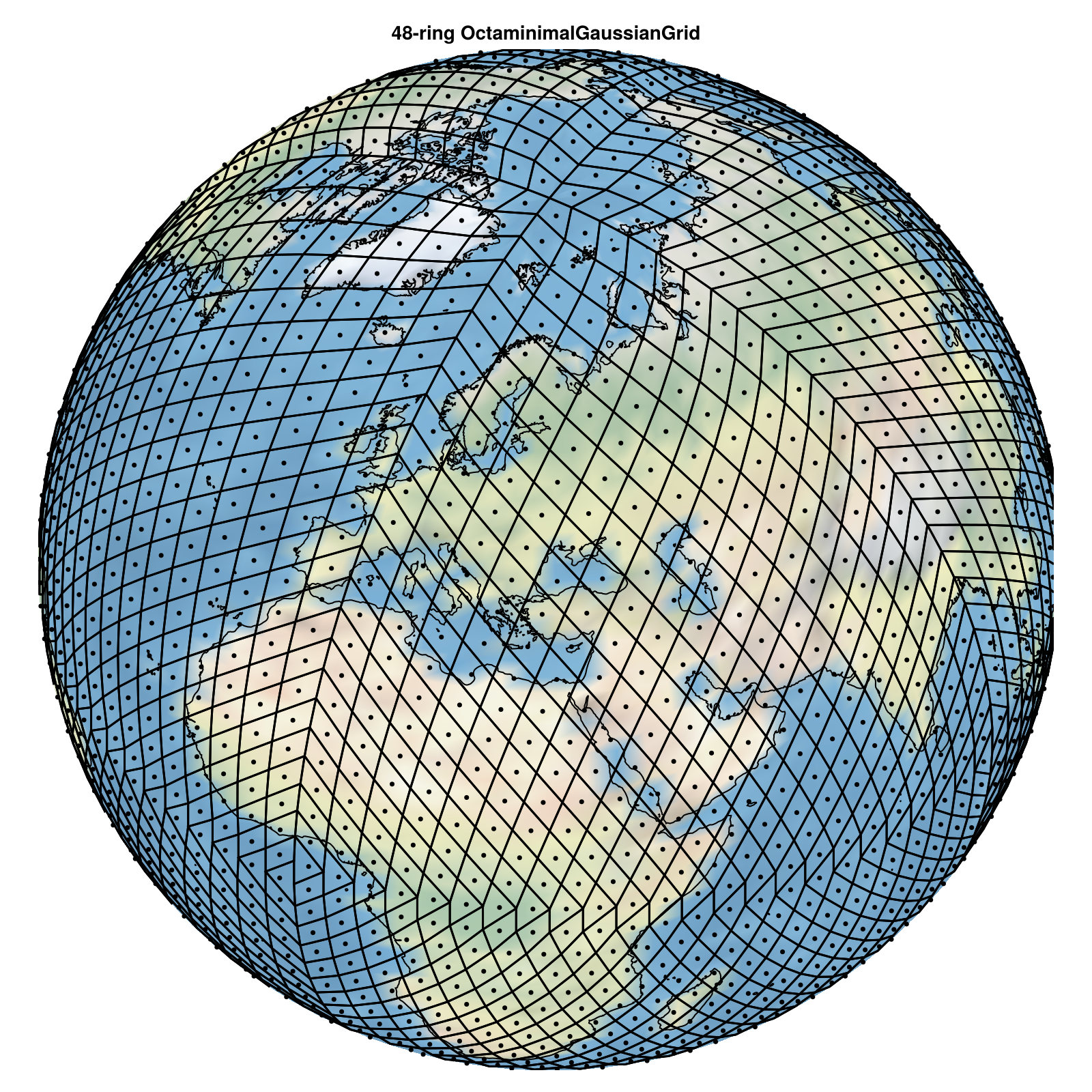

The OctaminimalGaussianGrid is similar to the OctahedralGaussianGrid but starts with 4 points around the poles. It therefore minimizes the number of grid points for the Gaussian grids at the cost of a (somewhat) inexact spectral transform. But for nlat_half = 24 (i.e. 48 latitude rings) this grid reduces the number of horizontal grid points from 3168 to 2400, i.e. -24% which speeds up the computation on the grid (dynamics and physics) as well as the spectral transform. The octaminimal Gaussian grid is intended to be used for low resolutions as for higher resolutions the relative increase in the number of grid points with the octahedral Gaussian grid becomes negligible.

Furthermore the longitudes are rotated: Instead of no offset where the first point on every ring starts at 0˚E, an offset of degrees is chosen similar to how the longitudinal points in the HEALPix grids (HEALPixGrid and OctaHEALPixGrid) are chosen. This allows for a more even distribution of grid points near the poles.

Full Clenshaw-Curtis grid

(called FullClenshawGrid)

using CairoMakie, GeoMakie    # when using GLMakie, use interactive=true (default) for zoom and rotation
globe(FullClenshawGrid, 24, interactive=false)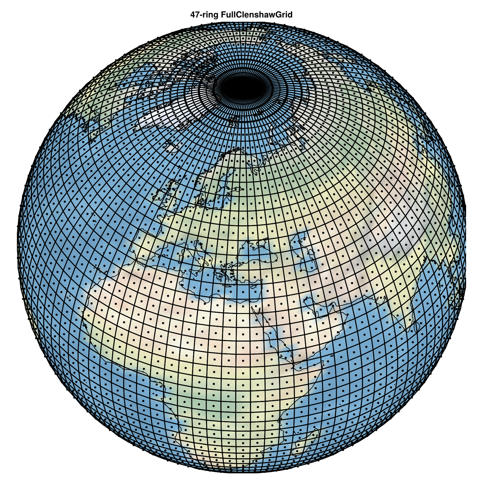

The full Clenshaw-Curtis grid is a regular longitude-latitude grid, but a specific one: The colatitudes , and the longitudes are

with the in-ring zonal index   and   the ring index starting with 1 around the north pole. There is no grid point on the poles, but in contrast to the Gaussian grids there is a ring on the Equator. The longitudes are shared with the full Gaussian grid. Being a full grid, also the full Clenshaw-Curtis grid suffers from too many grid points around the poles, this is addressed with the octahedral Clenshaw-Curtis grid.

The full Clenshaw-Curtis grid gets its name from the Clenshaw-Curtis quadrature that is used in the Legendre transform (see Spherical Harmonic Transform). This quadrature relies on evenly spaced latitudes, which also means that this grid nests, see Hotta and Ujiie[^HU18]. More importantly for our application, the Clenshaw-Curtis grids (including the octahedral described below) allow for an exact transform with cubic truncation (see Matching spectral and grid resolution). Recall that the Gaussian latitudes allow for an exact transform with quadratic truncation, so the Clenshaw-Curtis grids require more grid points for the same spectral resolution to be exact. But compared to other errors during a simulation this error may be masked anyway.

Octahedral Clenshaw-Curtis grid

(called OctahedralClenshawGrid)

using CairoMakie, GeoMakie    # when using GLMakie, use interactive=true (default) for zoom and rotation
globe(OctahedralClenshawGrid, 24, interactive=false)

In the same as we constructed the octahedral Gaussian grid from the full Gaussian grid, the octahedral Clenshaw-Curtis grid can be constructed from the full Clenshaw-Curtis grid. It therefore shares the latitudes with the full grid, but the longitudes with the octahedral Gaussian grid.

Notation as before, but note that the definition for only holds for the northern hemisphere, Equator included. The southern hemisphere is mirrored. The octahedral Clenshaw-Curtis grid inherits the exactness properties from the full Clenshaw-Curtis grid, but as it is a reduced grid, it is more efficient in terms of computational aspects and memory than the full grid. Hotta and Ujiie[^HU18] describe this grid in more detail.

HEALPix grid

(called HEALPixGrid)

using CairoMakie, GeoMakie    # when using GLMakie, use interactive=true (default) for zoom and rotation
globe(HEALPixGrid, 24, interactive=false)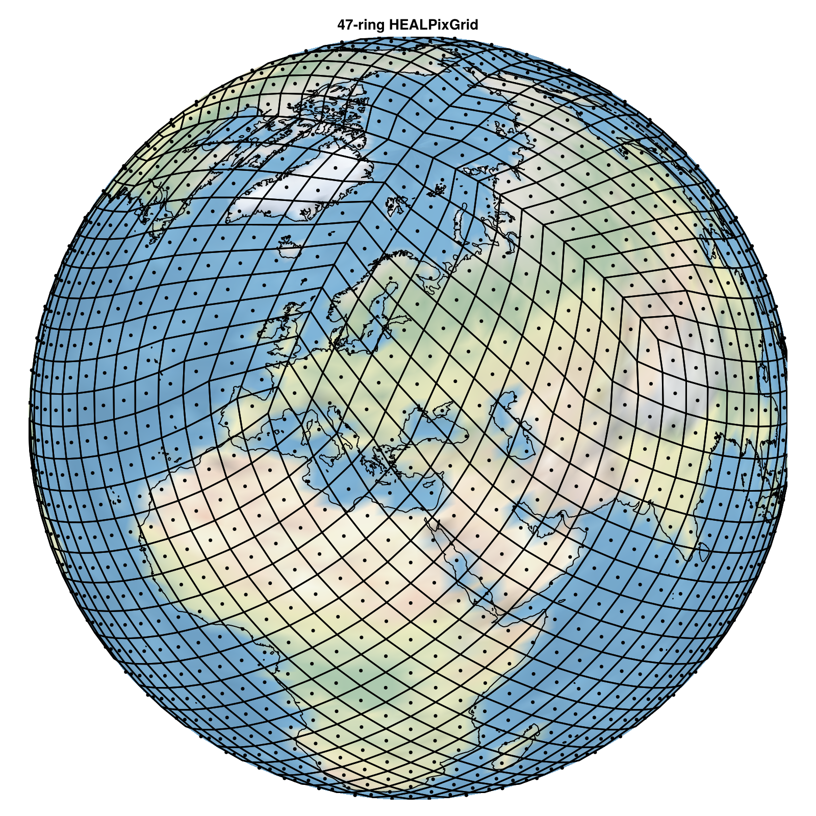

Technically, HEALPix grids are a class of grids that tessalate the sphere into faces that are often called basepixels. For each member of this class there are basepixels in zonal direction and basepixels in meridional direction. For   and   we obtain the classical HEALPix grid with   basepixels shown above in Implemented grids. Each basepixel has a quadratic number of grid points in them. There's an equatorial zone where the number of zonal grid points is constant (always , so 32 at  ) and there are polar caps above and below the equatorial zone with the border at   ( in colatitudes).

Following Górski, 2004[^G04], the   colatitude of the -th ring in the north polar cap,   with   is

and on that ring, the longitude of the -th point ( is the in-ring-index) is at

The in-ring index goes from   for the first (i.e. northern-most) ring,   for the second ring and   for the -th ring in the northern polar cap.

In the north equatorial belt   this changes to

and the longitudes change to ( is always   in the equatorial belt meaning the number of longitude points is constant here)

The modulo function comes in as there is an alternating longitudinal offset from the prime meridian (see Implemented grids). For the southern hemisphere the grid point locations can be obtained by mirror symmetry.

Grid cell boundaries

The cell boundaries are obtained by setting    or     (half indices) into the equations above, such that , a function for the cosine of colatitude of index and the longitude is obtained. These are then (northern polar cap)

with     and in the equatorial belt

OctaHEALPix grid

(called OctaHEALPixGrid)

using CairoMakie, GeoMakie    # when using GLMakie, use interactive=true (default) for zoom and rotation
globe(OctaHEALPixGrid, 24, interactive=false)

While the classic HEALPix grid is based on a dodecahedron, other choices for and in the class of HEALPix grids will change the number of faces there are in zonal/meridional direction. With   and   we obtain a HEALPix grid that is based on an octahedron, which has the convenient property that there are twice as many longitude points around the equator than there are latitude rings between the poles. This is a desirable for truncation as this matches the distances too, around the Equator versus between the poles.    or    are other possible choices for this, but also more complicated. See Górski, 2004[^G04] for further examples and visualizations of these grids.

We call the    HEALPix grid the OctaHEALPix grid, which combines the equal-area property of the HEALPix grids with the octahedron that's also used in the OctahedralGaussianGrid or the OctahedralClenshawGrid. As   there is no equatorial belt which simplifies the grid. The latitude of the -th isolatitude ring on the OctaHEALPixGrid is defined by

with  , and similarly for the southern hemisphere by symmetry. On this grid   where = nlat_half, the number of latitude rings on one hemisphere, Equator included, because each of the 4 basepixels spans from pole to pole and covers a quarter of the sphere. The longitudes with in-ring- index   are

and again, the southern hemisphere grid points are obtained by symmetry.

Grid cell boundaries

Similar to the grid cell boundaries for the HEALPix grid, the OctaHEALPix grid's boundaries are

The in the denominator of the HEALPix grid came simply for the OctaHEALPix grid and there's no separate equation for the equatorial belt (which doesn't exist in the OctaHEALPix grid).

References

[^G04]: Górski, Hivon, Banday, Wandelt, Hansen, Reinecke, Bartelmann, 2004. HEALPix: A FRAMEWORK FOR HIGH-RESOLUTION DISCRETIZATION AND FAST ANALYSIS OF DATA DISTRIBUTED ON THE SPHERE, The Astrophysical Journal. doi:10.1086/427976

[^M16]: S Malardel, et al., 2016: A new grid for the IFS, ECMWF Newsletter 146. https://www.ecmwf.int/sites/default/files/elibrary/2016/17262-new-grid-ifs.pdf

[^HU18]: Daisuke Hotta and Masashi Ujiie, 2018: A nestable, multigrid-friendly grid on a sphere for global spectralmodels based on Clenshaw–Curtis quadrature, Quarterly Journal of the Royal Meteorological Society, DOI: 10.1002/qj.3282